Tangential acceleration is the part of an object’s acceleration that acts along its path, changing its speed rather than its direction. It is measured in metres per second squared, and on a bend it sits at a right angle to the centripetal acceleration, so the total is the square root of the sum of their squares.
Ease off the brake as you turn into a roundabout and the car settles. Stay on it and the front tyres begin to complain. Nothing about the bend has changed in that moment — what has changed is that you are asking one set of contact patches to do two jobs at once.
Turning is one acceleration. Changing speed is another, and it acts at right angles to the first. Put the two together and the acceleration the car actually has stops pointing at the centre of the bend, and it grows.
What Is Tangential Acceleration?
Tangential acceleration is the acceleration an object has because its speed is changing, and it always lies along the path rather than across it.
Split the job in two and it becomes obvious. Holding a bend at a fixed speed needs an acceleration aimed inward, square to where you are going; that is the centripetal part, and our guide to circular motion physics covers it, its formula and its worked examples in full. Speeding up or slowing down needs an acceleration along the path instead.
Nothing says an object may only do one of them at a time. A car can hold a line through a bend and brake in the middle of it; so can a train, a cyclist, a rotor blade or a robot arm. Physicists call that non-uniform circular motion, and it is the ordinary case rather than the exotic one.
Its symbol here is at, and its unit is the metre per second squared, m/s2 — the same unit as any other acceleration. Worth pausing on that: the tangential component is not a different species of quantity. It is the same quantity pointing a different way.
The sign carries the meaning. Positive means the object is gaining speed along its path and negative means it is shedding it, and both are tangential acceleration. Whether the sign matters to the answer is a question the maths settles further down, and the answer is not the one most people expect.
The Tangential Acceleration Formula
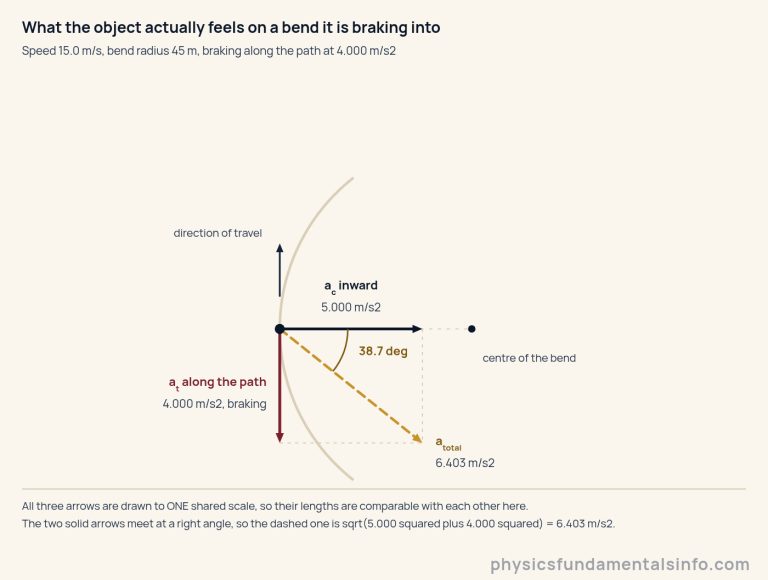
Because the two components meet at a right angle, the total acceleration is the hypotenuse of the triangle they make.
Every symbol in it is something you can measure at one instant:
- a — the total acceleration the object actually has, in metres per second squared (m/s2).
- ac = v2/r — the centripetal component, pointing at the centre of the bend, in m/s2. It is never negative.
- at — the tangential component, along the path, in m/s2. Negative means slowing down.
- v — the speed along the path at this instant, in metres per second (m/s).
- r — the radius of the bend, in metres (m), taken as constant.
The direction needs a second line, because a total on its own does not say where the acceleration points.
It is measured from the inward radius, and it runs from 0° when the speed is steady to 90° when the object is not yet moving but is already gaining speed, so every scrap of its acceleration lies along the path. Rearranged, the same relation returns whichever of the four quantities you are missing, and the tangential acceleration calculator runs all four modes with the centripetal part and the lean angle printed beside each answer.
One warning about running it backwards. Solving for at returns its size and not its sign, because the relation squares it — a limit of the information a total carries, not a shortcoming of the arithmetic.
The lab below draws the bend from above with all three arrows on it and a dashed circle showing the grip the manoeuvre is allowed. It opens on a steady bend, where the tangential arrow has nothing to draw: no lean, no dashed resultant and no angle marked. Move the tangential slider far enough off zero and the lean, the dashed resultant and the angle marker arrive together.
Read it with one caution. The drawing rescales itself so that whichever is longer, the resultant or the grip circle, always fills the same space — so an arrow’s length is a ratio within the screen in front of you, never a size to carry across to another setting. An arrow shorter than about three pixels is dropped rather than drawn, which is a limit of the picture and not of the physics.
How the Two Components Combine on a Bend
Perpendicular accelerations do not add end to end. They add in quadrature — squares, sum, square root — which is the whole reason a little braking is nearly free and a lot of it is not.
Take the bend in the diagram: 15.0 m/s round a radius of 45 m, so the inward component is 5.000 m/s2. Add 4.000 m/s2 of braking along the path and the total climbs to 6.403 m/s2, leaning 38.7° off the inward radius. The inward component has not moved at all; only the total has.
Now watch how cheap the first slice is. Start from an inward component of 7.000 m/s2 and hang a whole 1.000 m/s2 of braking on it: sqrt(49.000 + 1.000) is 7.0711 m/s2. A seventh has been added to one side of the triangle and the hypotenuse has grown by 1.015 per cent.
Push harder and the bargain disappears. At 5.000 m/s2 of braking the total reaches 8.6023 m/s2, 22.890 per cent up on where it started. Squaring is unforgiving once the second component stops being small compared with the first.
There is one exact landmark on the way. Equality has a speed of its own: set v2/r against the size of at and the two match at v = sqrt(at r), where the lean is exactly 45°. For the braking case above, a 45 m radius with 4.000 m/s2, that works out at 13.416 m/s.
Do not file that figure as a constant. It moves with both the radius and the tangential acceleration: on a 20 m bend with 2.500 m/s2 it is 7.071 m/s instead. Nor does the starting speed enter it anywhere, so the crossover belongs to the bend and the manoeuvre and not to how the journey began. OpenStax University Physics sets out the same decomposition, with the total acceleration as the vector sum of two perpendicular parts.
The Grip Budget: What Braking Costs Your Cornering Speed
Everything above is geometry and holds for any object on any curved path. Tyres add one more fact, and it is the fact that makes the geometry matter: the surface can only supply so much acceleration in total, and turning and speed-changing draw on the same account.
Write that ceiling as the grip coefficient times g, with g = 9.81 m/s2. Static friction has a maximum of the coefficient times the normal force, OpenStax’s chapter on friction sets that out, and it is equally plain that the model is an approximate empirical one whose coefficient depends on the two surfaces in contact. Treat the coefficient here as a number you choose, never as a measurement of any particular road.
Pick 0.80 and the budget is 0.80 × 9.81 = 7.848 m/s2. The steady bend above uses 5.000 of that, or 63.7 per cent. Brake at 4.000 m/s2 in the middle of it and the total of 6.403 uses 81.6 per cent — still inside the budget, but with far less left over.
Drawn out, that budget is a circle, and the two components are coordinates on it.
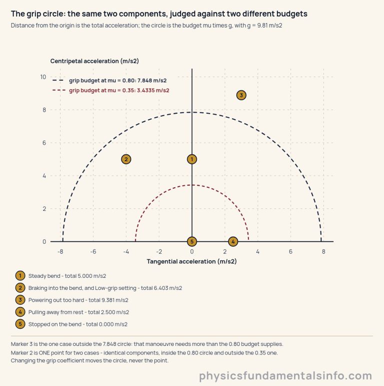
That picture is the mechanism behind a line most drivers already know: braking hard in a corner is how you lose grip. The braking does not make the corner harder. It enlarges the demand on the surface, and the circle says by exactly how much.
It also puts a number on what you give up. If you spend a fraction x of the budget changing speed, the fastest you could still take that bend falls to (1 − x2)1/4 of what it was.
| Grip budget spent changing speed | Cornering ceiling you keep | Cornering ceiling you lose |
|---|---|---|
| 0 per cent | 100.00 per cent | 0.00 per cent |
| 10 per cent | 99.75 per cent | 0.25 per cent |
| 25 per cent | 98.40 per cent | 1.60 per cent |
| 50 per cent | 93.06 per cent | 6.94 per cent |
| 75 per cent | 81.33 per cent | 18.67 per cent |
| 90 per cent | 66.02 per cent | 33.98 per cent |
| 99 per cent | 37.56 per cent | 62.44 per cent |
Read the third column slowly, because it is the point of the table. A quarter of your grip spent on braking costs 1.60 per cent of the ceiling; half of it costs 6.94 per cent; nine tenths costs a third. The penalty is almost nothing at first and then arrives all at once.
Be precise about what is falling, though. This is the ceiling coming down, not the car slowing: a driver at 15 m/s who brakes hard is not suddenly doing 6.94 per cent less. The fastest that bend would have allowed has dropped, and how close the driver was to it is a separate question.
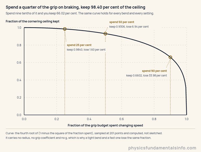
And here is the detail that lifts this above a rule of thumb. That fraction contains no radius, no coefficient and no g — so a 45 m bend at 0.80 and a 200 m bend at 0.35 both keep 0.930605 of their ceiling when half the budget goes on changing speed. Problem 8 works both.
Real-World Examples of Tangential Acceleration
Braking into a corner. A driver arriving at a bend is rarely at a settled speed. Every bit of brake carried past the turn-in point is a tangential acceleration sharing the surface with the inward one, which is why coaches talk about bleeding the brake off as the steering goes on. The grip circle above is the picture behind that advice.
Anything spinning up. A point on a grinding wheel, a centrifuge rotor or a turbine disc travels a circle of fixed radius. While the machine is getting up to speed, that point carries both components at once; once the speed settles, the tangential one vanishes and only the inward one is left.
Trains and trams leaving a curve. Rail vehicles routinely accelerate while still on a curve. The wheels must supply the inward force that holds the curve and the forward force that builds the speed, and it is their combination the track and the contact patch have to carry.
Machine tools and robot arms. Curve the path of a tool head and then change how fast it runs along that path, and both components are live at once. The limit the drive has to respect is the combined figure, which is why path planners budget for a total and not for a turning rate and a feed rate separately.
One thread runs through all four. Nobody is arguing about whether the object is turning or whether it is changing speed. They are counting what the two together demand.
Common Misconceptions About Tangential Acceleration
“a = v2/r must be wrong if the speed is changing.” It is not wrong, and this is the most important sentence on the page. It gives the centripetal component, and that component is exactly right whatever the speed is doing. What it does not give is the whole acceleration, because a second component has appeared along the path and the formula has no slot for it.
“Braking costs more grip than accelerating.” Not in this model. The tangential term enters as a square, and a square cannot tell a minus sign from a plus one, so shedding 4.000 m/s2 and adding 4.000 m/s2 land on the same total and the same lean. Braking is the classic way to lose a corner because braking is what drivers do there, not because the physics charges a premium for it.
“Spend half your grip on braking and you lose half your cornering speed.” You lose 6.94 per cent of the cornering ceiling. Quadrature is why: half the budget spent on one axis leaves the square root of three quarters for the other, and then a further square root to turn an acceleration ceiling into a speed ceiling.
“Tangential acceleration is just the ordinary acceleration you already know.” Nearly, and the gap matters. It is one component of the acceleration, picked out by direction, and calling the whole vector by that name loses the inward part — which on our worked bend is the larger of the two. Direction is what separates them, as any treatment of scalar and vector quantities insists.
How Tangential Acceleration Relates to Circular Motion and Angular Acceleration
This page adds one member to a family the rest of the site already covers, and changes none of the others.
Start with the uniform world. Everything in circular motion physics — the definition of centripetal acceleration, a = v2/r, the symbol table and the three equivalent forms — holds exactly as written the moment the speed stops changing, which is most of the time. Reach for the circular motion calculator while the speed holds still; it carries no tangential box, and with a fixed speed there would be nothing to type into one.
Then the rotational view. Divide the speed by the radius and you have the angular velocity ω; divide the tangential acceleration by the radius and you have the angular acceleration α. The same two components reappear as ω2r and αr, which is the language the angular velocity guide works in.
Those two forms are substitutions rather than independent checks, and it is worth saying so plainly. Writing v = ωr and then finding that ω2r equals v2/r is algebra agreeing with itself, not evidence about the world.
Force is one multiplication away. Multiply either component by the mass and you have the force that produces it, which is where centripetal force and its distinction from centripetal acceleration belong; that page settles it and this one assumes it.
If you would rather push the sliders than read, the tangential acceleration simulator is the same lab on a page of its own, with worked cases to load and a caption that changes when the lean disappears.
Where This Model Breaks Down
The relation itself is exact. What can fail is pressing it onto a motion it does not describe, and there are five honest limits worth naming.
The grip circle is an idealisation. A real tyre’s limit is not a perfect circle, it changes with load and temperature, and this model knows none of that. It is a good first picture of a shared budget and a poor description of any actual tyre.
The coefficient is an input, not a measurement. Nothing on this page, in the lab or in the calculator measures a surface; every figure quoted here is the consequence of a coefficient somebody typed in. Compare the result with a figure you trust for the surface in front of you, and make that comparison yourself.
The readouts are a snapshot. at is the rate of change of speed at one instant, so nothing here integrates a lap or a manoeuvre forward in time; the radius is fixed too, which rules out a corner that tightens and any transition curve. And the path is taken to be level, so a banked bend is a different calculation — the banked curve calculator covers that one.
A last word on evidence. This article, the lab and the calculator all run the same relation, so their agreeing with one another proves only that one piece of algebra was implemented three times. What is worth testing is out on a road or a rig, with a stopwatch rather than a screen.