A superconductor is a material that, below a critical temperature, carries electric current with no measurable resistance and expels magnetic field from its interior. That state has three limits and crossing any one ends it: the critical temperature, the critical magnetic field, and the critical current that field allows the wire to carry.
Set a current running round a closed loop of superconducting wire, disconnect the battery and walk away. The current keeps going. In a superconducting gravimeter in Belgium one did exactly that for 10467 days — twenty-eight years, seven months and twenty-seven days — with no decay anyone could detect.
Most explanations stop there, at “the resistance falls to zero”. Zero, though, is a limit rather than a measurement, and it leaves the three questions a physicist actually asks unanswered: how cold, how much magnetic field, and how much current. This page answers all three with numbers.
What Is a Superconductor?
A superconductor is a material that, cooled below its critical temperature, carries a current with no measurable resistance and drives magnetic field out of its own interior.
Two properties, not one. Students often learn the first and forget the second, and the second is the one that makes the topic behave strangely. Cooling a perfect conductor would trap whatever field happened to be inside it; a superconductor instead pushes the field out, which is a different and stronger statement.
That expulsion is the Meissner effect, and it is why the topic has a limit at all. Pushing a field out costs energy, and the material only has so much to spend. Turn the applied field up far enough and the superconducting state is simply no longer worth having, so it stops.
The temperature at which it stops with no field applied is the critical temperature, Tc. Lead’s is 7.19 K. That is 7.19 degrees above absolute zero, which is why almost every sentence about this topic quietly assumes a cryostat in the room.
Ordinary metals have no such point. Cool copper and its resistance falls smoothly, flattening out at a residual value set by impurities and never reaching zero. A superconductor does something categorically different at Tc: it changes phase, and Ohm’s law stops having anything to say, because there is no longer a resistance to multiply the current by.
Materials divide into two families. Type-I superconductors, which are mostly pure elements, expel field completely until one critical field destroys the state outright — and everything computed on this page is type-I. Type-II materials, which is what real magnets are wound from, let flux through in quantised threads over a wide band of field and survive far higher fields as a result.
Is a Superconductor’s Resistance Really Zero?
No experiment can measure zero, so the honest answer is an upper bound rather than a value: on the longest measured persistent current, the loop’s resistance is below roughly 1.1 × 10⁻¹⁸ ohms.
Here is where that comes from. A current circulating in a loop of inductance L against a resistance R decays as I(t) = I0e−Rt/L. Rearranging for R gives an inequality, because what an experiment actually establishes is that the current did not change by more than some detectable fraction f.
- R — the upper bound this places on the loop’s resistance, in ohms (Ω).
- L — the loop’s inductance, in henries (H). A stated assumption, not a measurement.
- t — how long the current was watched for, in seconds (s). This is the sourced part.
- f — the largest fractional decay the apparatus could have missed, a pure number. Also a stated assumption.
The 10467 days is the sourced number, from the record of persistent currents in superconductivity. Put it in with a 1 mH coil and a detection floor of one part in a million — both of which are assumptions you are free to change — and the bound lands at 1.10576859 × 10⁻¹⁸ Ω. Problem 8 below does that arithmetic line by line.
Turn it into a resistivity and the scale becomes easier to feel. For a 0.5 mm-radius wire, 100 m of it, that bound is 8.6846862 × 10⁻²⁷ Ω m. Copper, at the 1.68 × 10⁻⁸ Ω m this site publishes in its resistivity calculator, is more resistive than that by a factor of 1.934439 × 10¹⁸.
So “zero” is not quite the claim. The claim is bounded, and bounded so far below every other material that the difference has no experimental consequence. Our guide to electrical resistance asks in its own FAQ whether resistance can ever be zero; this is the number that answer was missing.
There is a second reason the decay is not gradual. Flux through a superconducting ring comes in whole multiples of the magnetic flux quantum, and the NIST value of that magnetic flux quantum is 2.067833848 × 10⁻¹⁵ Wb exactly. Since the flux is L times the current, the current in a 1 mH ring can only change in steps of 2.07 pA.
A bigger magnet has a smaller step, because the step is the flux quantum divided by L: for a 100 H coil it is about 20.7 attoamps. There is no smooth way down, which is the real content of “zero resistance”.
Be careful with what that does and does not prove. It removes the gradual path, not the possibility — a large enough fluctuation can still move the whole loop by one quantum. That is precisely why every measured lifetime is quoted as a bound and never as an infinity.
The Superconductor Formulas: Critical Field and Critical Current
Two relations carry all the quantitative content, and they are on very different footings. The first is a fit; the second is a derivation.
- Bc(T) — the critical magnetic flux density at temperature T, in tesla (T). Above it the metal is an ordinary conductor.
- Bc0 — the same quantity extrapolated to absolute zero, in tesla (T). Lead’s is 80 mT.
- T — the operating temperature, in kelvin (K).
- Tc — the critical temperature, in kelvin (K), where the critical field reaches zero.
That parabola is empirical. It is the standard fit for type-I elements, good to a few per cent, and nothing on this site derives it; two endpoints and a monotonic fall between them are the whole of its claim.
Notice, though, that it meets the temperature axis at a finite angle rather than flattening into it. Superconductivity does not fade away as you warm towards Tc. There is a last field it will hold, right up to the end.
The second relation turns that field into a current, and it is the one exact step in the chain.
- Ic — the critical current, in amperes (A). Above it the wire goes normal.
- a — the wire’s radius, in metres (m). Not its diameter, and this is the commonest slip in the whole topic.
- Bc(T) — the critical field at the working temperature, in tesla (T), from the parabola above.
- μ0 — the permeability of free space, 1.25663706212 × 10⁻⁶ N/A² here, in newtons per ampere squared.
This is Silsbee’s rule, and it is worth saying plainly that it is derived rather than fitted. It inherits the parabola’s few-per-cent error and adds none of its own, which also means a critical current quoted to six figures is precise rather than accurate. Rearranged, the same relation answers a designer’s questions instead of a student’s: how cold, how thin, or what field a target current needs. Our superconductor critical field calculator solves it in any of those directions and prints the critical field, the current density and the penetration depth beside the answer.
One consequence of the formula is easy to miss and worth pinning down now. The wire’s own current puts a magnetic field on its own surface, and the material cannot tell that field apart from one you apply from outside.
Run 100 A through a 0.5 mm-radius lead wire in no applied field, or run no current at all through the same wire sitting in a 40 mT field, and the metal sees the identical surface field and has the identical margin left. Both cases eat the same budget. An applied field is therefore not a separate hazard from a large current — it is the same hazard, arriving from a different direction.
The simulator below is that budget, made adjustable. Set the material’s two numbers, the temperature, the applied field, the transport current and the wire radius, and it plots the operating point against the critical-field curve, draws the field’s decay into the metal, and tells you which side of the boundary you have landed on.
Here is that boundary on its own, drawn once for lead. The simulator’s main panel is this same picture with an operating point loose inside it.
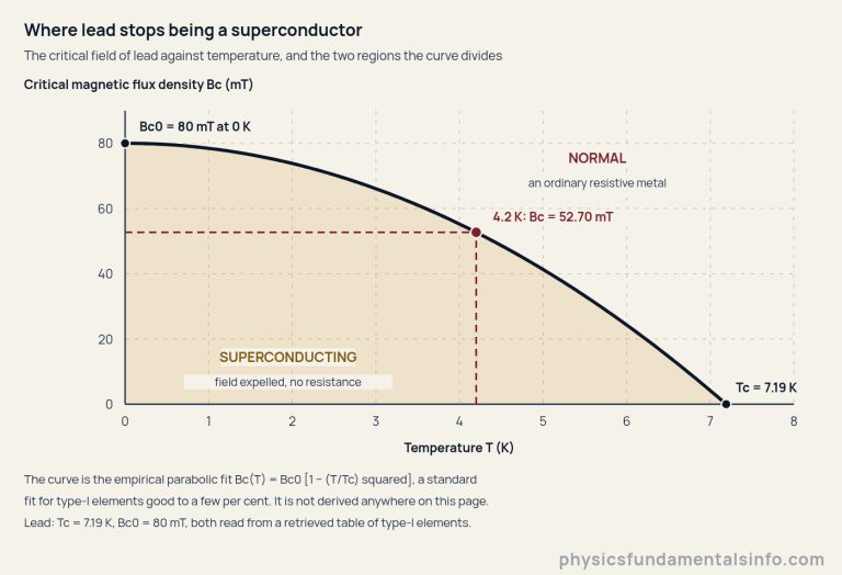
How Silsbee’s Rule Follows from Ampère’s Law
The derivation is two lines, and following it is the difference between quoting the formula and understanding what it claims.
Take Ampère’s law round a circle drawn on the surface of a round wire of radius a carrying current I. The enclosed current is I and the path length is 2πa, so B × 2πa = μ0I, giving a surface field of B = μ0I/(2πa). No approximation has been made; this is exact for a round wire.
Now add the physics. The material expels field until the field at its own surface reaches Bc(T), and at that point it gives up. Set μ0Ic/(2πa) = Bc(T), rearrange, and Silsbee’s rule drops out with no fitted constant anywhere in it.
The arithmetic hands you a shortcut worth keeping. Because μ0/(2π) is 2.000000001089 × 10⁻⁷, the surface field of a round wire in millitesla is very nearly 0.2 × I(A) / a(mm) — so 100 A in a 0.5 mm-radius wire is 40 mT, done in your head.
Do not call that an identity. It was one before 2019, when μ0 was defined as 4π × 10−7; the SI redefinition made the permeability a measured quantity, and NIST’s current vacuum magnetic permeability agrees with the value used here to nine significant figures. Excellent approximation, not an equality.
Look at what the rule says about size and something counter-intuitive falls out. The critical current is proportional to the radius, not to the area, because the quantity that kills the wire lives on the surface. Four times as much metal buys exactly twice the current.
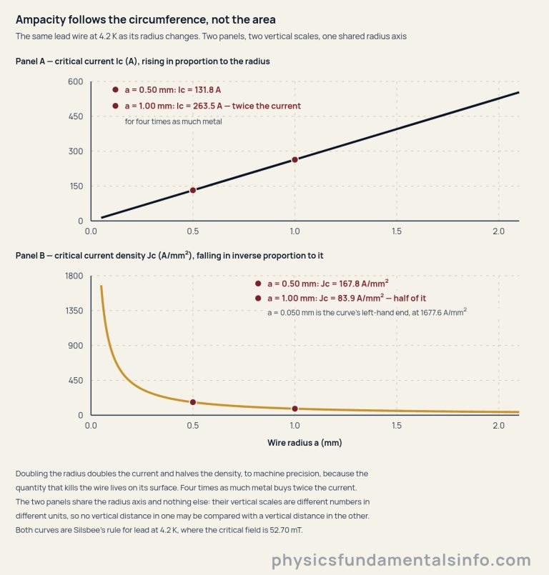
The copper comparison has to name which copper rule it is contrasting, because there are two. At a fixed current density, copper’s ampacity goes as the area and therefore as the square of the radius, and that is the rule of thumb being overturned here. At a fixed watts-per-metre limit, copper scales with the radius too, so the contrast would be no contrast at all.
The same result says something blunter about the middle of a superconducting wire: it does nothing. Silsbee’s rule sees only the outer radius, so a tube of the same outer radius carries exactly the same critical current as a solid rod, on a small fraction of the metal.
Problem 7 works the figure out. A 0.5 mm-radius tube with a 1 µm wall matches the solid rod on 0.3996 per cent of the lead, a saving of over 250 times, which is why real superconducting cable is thousands of fine filaments in a normal-metal matrix rather than one thick rod. The wall cannot shrink for ever, and the next section says exactly where it has to stop.
Critical Temperature and Critical Field of the Type-I Elements
Eleven elements carry both numbers in the table retrieved for this cluster, and they are the complete legal material space for every calculation on this page.
| Element | Critical temperature Tc (K) | Critical field at 0 K, Bc0 (mT) |
|---|---|---|
| Lead (Pb) | 7.19 | 80 |
| Tantalum (Ta) | 4.48 | 90 |
| Mercury (α-Hg) | 4.15 | 40 |
| Tin (Sn) | 3.72 | 30 |
| Indium (In) | 3.4 | 30 |
| Thallium (Tl) | 2.39 | 20 |
| Aluminium (Al) | 1.20 | 10 |
| Gallium (Ga) | 1.083 | 5.8 |
| Zinc (Zn) | 0.855 | 5 |
| Cadmium (Cd) | 0.52 | 2.8 |
| Titanium (Ti) | 0.39 | 10 |
Read the two columns against each other and the table says something a single ranking would hide. Tantalum has a lower critical temperature than lead, 4.48 K against 7.19 K, and yet a higher critical field, 90 mT against 80 mT.
Titanium makes the same point harder. It tolerates the same 10 mT as aluminium while transitioning at 0.39 K, barely a third of aluminium’s 1.20 K. Ranking materials by critical temperature alone is therefore wrong, and these numbers say so rather than an opinion saying so.
Real magnets are not wound from any of them. They use type-II materials, whose field column is a genuinely different quantity: the upper critical field Bc2, above which superconductivity finally ends, with a broad band below it in which flux threads through the material and the state survives anyway. Neither the parabola nor Silsbee’s rule applies to the rows below, and this page never applies them there.
| Type-II material, for context only | Critical temperature Tc (K) | Upper critical field Bc2 (T) |
|---|---|---|
| Niobium (Nb) | 9.26 | 0.82 |
| Niobium–titanium (NbTi) | 10 | 15 |
| Niobium–tin (Nb3Sn) | 18.3 | 30 |
| Magnesium diboride (MgB2) | 39 | 74 |
| YBCO cuprate | 95 | 120 to 250 (a range) |
YBCO gets a range and not a number because the source gives a range, and inventing a midpoint would be the kind of tidy-looking fiction this page exists to avoid.
The last column of that table is also the whole reason the cuprates caused a fuss. Liquid nitrogen boils at 77.36 K and liquid helium at 4.22 K, two figures our article on absolute zero and the temperature scale already publishes. On the sourced numbers exactly one row here — the 95 K cuprate — can be cooled with nitrogen. Everything else, magnesium diboride included, needs something colder than nitrogen.
Where This Superconductor Model Stops Working
Three things break this model, and each of them has a measurable boundary rather than a vague warning. A fourth heading below simply lists what was never sourced at all.
The parabola is a fit, and so is the penetration depth
Every critical field on this page rests on an empirical parabola that nothing here derives, and the same goes for the temperature dependence of the penetration depth, λ(T) = λ0/sqrt(1 − (T/Tc)4). Both are standard fits for type-I elements. Silsbee’s rule sitting on top of them is exact, so the answers carry the fits’ error and no more.
Why a thin enough wire breaks it
Share the critical current out over the whole cross-section and you have a density, Jc = 2Bc/(μ0a). Shrink a towards nothing and that expression climbs without bound, promising any current density you care to name from a fine enough filament. No metal can honour that, so somewhere the arithmetic has run past the physics.
Where it runs past it is fixed by the only length a superconductor owns, the penetration depth. Screening the critical field across a depth λ needs a density of about Bc/(μ0λ), and that bare field scale carries no fitted coefficient of any kind.
Set the two equal and the crossing falls at a = 2λ exactly, independently of material, field and temperature. Taking 100 nm as the order of magnitude for λ, a 1 mm-diameter wire sits 2500 times below that scale, which is comfortable. The 5 µm filaments inside real cable sit only about 12.5 times below it, which is precisely where a page should stop quoting the rule as if it were the answer.
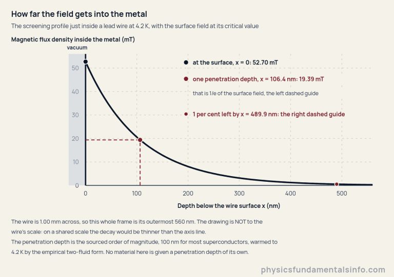
The penetration depth runs away at the critical temperature
Silsbee’s rule quietly assumes the current hugs a surface, and λ(T) diverges at Tc, so the rule must die once the screening depth reaches the wire’s radius. Solving for that temperature gives a window, and for a wire you can hold the window is absurdly thin: for a 0.5 mm-radius lead wire it is 71.9 nanokelvin wide.
The divergence is real and, at that width, irrelevant. For a 2.5 µm-radius filament the same window opens to 2.88 mK, about forty thousand times wider, and that is the direction that matters.
What this cluster did not source, and therefore never states
No material on this page is given a penetration depth of its own: 100 nm is the published order of magnitude for most superconductors, and it is used as an order and nothing finer. No coherence length, carrier density, molar mass or low-temperature heat capacity appears for any material either, because none was sourced.
Nor is anything claimed here about superconductivity at or near room temperature. Nothing was sourced for it, so nothing is said.
Real-World Examples of Superconductors
The state turns up in three places most readers have already met: a lecture bench, a hospital corridor, and a very long spool of wire.
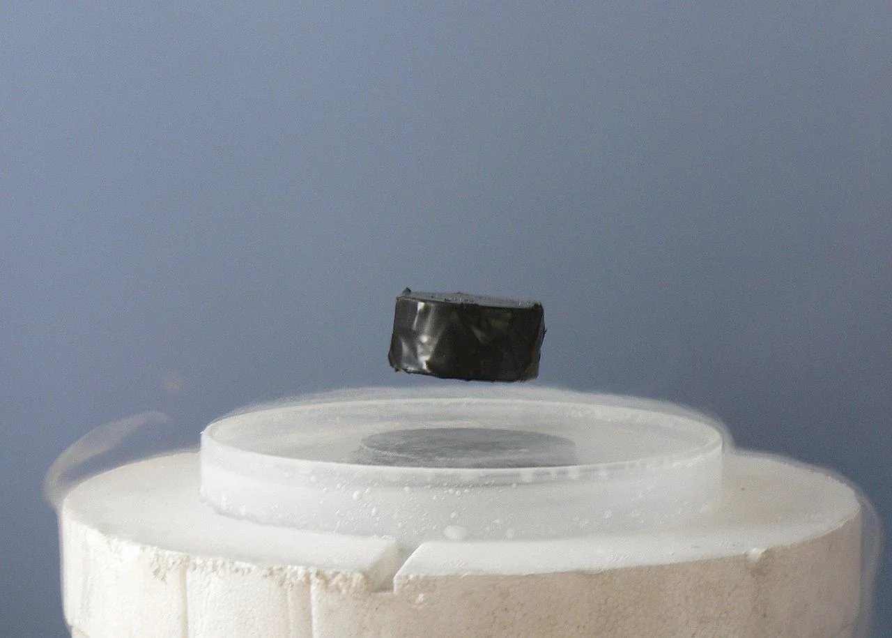
The floating magnet on the lecture bench
A small magnet hanging in mid-air above a chilled disc is the image nearly everyone has of this topic, and it is a real effect. It is not, however, the effect this page computes. The magnet is held by flux pinned inside a type-II material, which is a different mechanism from the complete field expulsion modelled here, so no number on this page describes that demonstration.
Scanner magnets, and why they are not made of lead
A medical scanner’s bore is a very large superconducting solenoid carrying an enormous current with no resistance, and our article on the electromagnet already notes that tens of tesla are a superconducting speciality. Those coils are type-II, for a reason the energy makes obvious.
The condensation energy density of lead, the free-energy advantage that makes the superconducting state worth having, is 2546.5 J/m³ at absolute zero. A 1 T field carries 397887.4 J/m³, which is 156.25 times as much, and that ratio is exactly (1 T / 80 mT) squared. A lead coil would destroy itself long before it became a useful magnet.
That advantage is also startlingly small in thermal terms. A cubic centimetre of lead holds 2.546479 mJ of it and weighs 11.34 g; at lead’s room-temperature specific heat that is the heat needed to warm it by 1.754 mK. Heat capacity falls steeply on cooling, so the true figure at 4 K is larger than that — the honest statement is a lower bound, because no low-temperature heat capacity was sourced here.
Cable, and the price of resistance in watts
Here is what the whole business buys, in units an electrician would recognise. A 1 mm-diameter lead wire at 4.2 K carries 131.8 A with nothing dissipated at all. The same wire in copper, carrying the same current, burns 371.3 W for every metre of it — roughly a hot plate per metre of cable.
Double the radius and something neat happens. The critical current doubles, and copper’s loss at that new current is unchanged at 371.3 W/m, because the current squared quadruples exactly as the resistance per metre quarters. Silsbee’s rule and Joule’s law move in lockstep there.
Common Misconceptions About Superconductors
“A superconductor has exactly zero resistance”
It has no measurable resistance, which is a different and weaker claim, and the difference is the whole of section two. The strongest statement any experiment supports is a bound — about 1.1 × 10⁻¹⁸ Ω on the stated assumptions — not a zero.
“The critical temperature is the number that matters”
Tantalum quenches at a lower temperature than lead and survives a stronger field. Titanium matches aluminium’s field tolerance from a third of the temperature. A material has at least two numbers, and a design that ignores the field column will fail in a magnet while looking fine on paper.
“A thicker superconducting wire carries proportionally more current”
Four times the metal buys twice the current, because the critical current follows the circumference rather than the area. The rule of thumb being overturned is copper’s fixed-current-density one, not copper’s thermal limit, which also scales with the radius.
“A modest applied field costs a modest slice of the current”
It does not. Because the critical current is linear in the headroom left over, the fraction of the rating a field costs is exactly the fraction of the critical field it takes. Problem 4 puts a 30 mT field on lead at 4.2 K and watches 56.9 per cent of the current rating disappear.
“A persistent current runs for ever”
It runs until something moves the trapped flux by one quantum, and nothing on this page rules that out. Flux quantisation removes the smooth path downward; it does not remove the possibility. Twenty-eight years of no detectable change is a magnificent bound and still a bound.