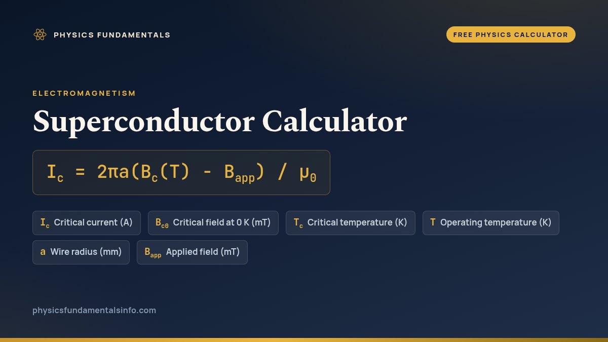
A superconductor is a material that below a critical temperature loses all measurable electrical resistance and expels magnetic field from its interior. This free superconductor calculator answers the question that follows: how much current will such a wire carry before it goes normal again? Type a critical field, a critical temperature, an operating temperature, a wire radius and any applied field, and it returns the critical current from Ic = 2πa(Bc(T) − Bapp) / μ0, with the critical field at your temperature, the current density, the penetration depth and what the same wire would cost in copper printed beside it.
Load a real metal
Every button moves the Solve for menu to whichever quantity its own case leaves unknown, sets each unit menu it names, and types the remaining figures. The line underneath quotes back whatever the widget works out from that, so nothing in it is stored text. The first five run forwards on sourced type-I elements; the last four read the same relation backwards, one for each of the other four modes.
Pick a case above, or type your own numbers.
What Is the Superconductor Calculator?
The superconductor calculator is a free online tool for the current a superconducting wire carries with no resistance at all. Enter the critical field at absolute zero, the critical temperature, the temperature the wire is held at, its radius and any applied field, and it returns the critical current from Ic = 2πa(Bc(T) − Bapp)/μ0, together with the critical field at that temperature, the critical current density, the penetration depth as an order of magnitude, the condensation energy density and what the same wire would waste in copper carrying the same current. Point the Solve for menu at the radius, the critical field, the operating temperature or the critical temperature instead and it rearranges the same relation, so a demanded current gives back the temperature it needs.
The two relations behind it are on a different footing and the page says so. Bc(T) = Bc0[1 − (T/Tc)2] is an empirical fit, the standard one for type-I elements and good to a few per cent, while Silsbee’s rule is derived in two lines from Ampère’s law and adds no error of its own. Two results are physical zeros rather than errors: at or above the critical temperature, and with an applied field at or above the critical field, the critical current is exactly zero, and a worded chip says which of the two it is. The model is a single round type-I wire, so type-II materials such as niobium-titanium and the cuprates appear on the page as a labelled context table only, with no formula applied to them.
| Symbol | Quantity | Default unit | Also accepts | Example value |
|---|---|---|---|---|
| Ic | Critical current | A | kA, mA | 131.7550066 |
| Bc0 | Critical field at 0 K | mT | T, G | 80 |
| Tc | Critical temperature | K | — | 7.19 |
| T | Operating temperature | K | — | 4.2 |
| a | Wire radius | mm | m, um | 0.5 |
| Bapp | Applied field | mT | T, G | 0 |
How to use the superconductor calculator
- Choose the unknown. The Solve for menu opens on Critical current. The other four choices are Critical field at 0 K, Critical temperature, Operating temperature and Wire radius, and whichever you pick vanishes from the boxes below.
- Type the critical field at 0 K. This box takes mT, T or G and opens on 80 mT, which is lead. It is the field extrapolated to absolute zero rather than the field at your working temperature, and it must be above zero: a material with no critical field never superconducts at all.
- Type the critical temperature. Critical temperature is in K and nothing else, and it opens on 7.19 K. It must be above zero, because a critical temperature of zero divides the parabolic law by zero and hands back a field of minus infinity.
- Type the operating temperature. Operating temperature is also in K, and it opens on 4.2 K because liquid helium boils at 4.22 K. Zero is legal and means absolute zero; at or above the critical temperature the answer is
0 Arather than a refusal, because the metal is simply a normal conductor there. - Type the wire radius. Wire radius takes mm, m or um and opens on 0.500 mm, which is a wire 1 mm across. It is the radius and not the diameter, and typing 1 mm there doubles the answer from 131.755 A to 263.51 A — the single commonest mistake on this page.
- Type the applied field. Applied field takes mT, T or G and opens on zero. It can never be the unknown and it can never be negative, because it eats into the same field budget the wire needs for its own self-field.
- Read the answer. The headline carries six significant figures while it stays a plain decimal and becomes a four-figure exponential outside that range. The answer box shows whichever unit its own menu is set to, so a current reads in amps, kiloamps or milliamps, and
0is a real answer rather than a failure. - Read the nine chips. They give the critical field at your temperature, the critical current density, the penetration depth as an order of magnitude, the condensation energy density, the reduced temperature, the headroom left for the self-field, what the same wire would cost in copper, how far the state sits from the limit of Silsbee’s rule, and a worded summary of what this state means.
- Open Show working. The steps run the empirical parabolic law first and the derived Silsbee step second, print your figures in the units the arithmetic really uses, and show the unrounded answer beside the rounding the headline applies to it. Every reverse mode also checks itself forwards.
Three calculators here already own the neighbouring questions, and none of them can answer this one. The resistivity calculator is R = ρL/A, the geometry of a wire, and it is where the 1.68e-8 Ω m copper figure used on this page comes from; the magnetic field calculator gives B = μ0nI inside a solenoid rather than the field at the surface of a single round wire. Ohm’s law presumes there is an R to divide by, which is exactly what a superconductor takes away.
That gap is why this page exists. The guide to electrical resistance tells the reader that resistance falls to zero in a superconductor and promises the persistent-current result in its own FAQ, without saying how cold, how much field or how much current; the six-line derivation, the drawn phase diagram and eight worked problems are in the guide to superconductors, which this tool is the arithmetic half of.
Two mistakes account for most wrong answers here. The first is typing a diameter where a radius belongs, which doubles or halves the answer without looking like a slip. The second is re-deriving the current by hand from the printed critical field: at 4.2 K the chip reads 52.70 mT, and putting that rounded figure back through Silsbee’s rule gives 131.750 A where the exact chain gives the 131.755 A the headline shows.
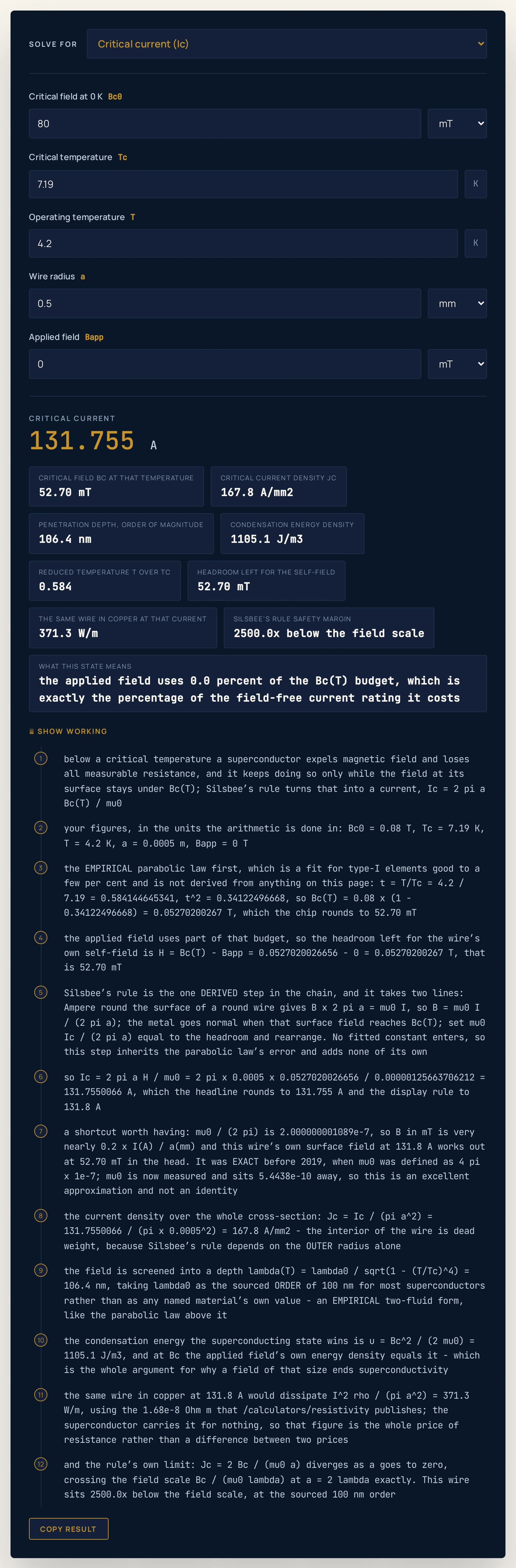
52.70 mT at 4.2 K becomes 131.755 A of critical current, and the same wire in copper would burn 371.3 W/m carrying it.Worked example: change one thing at a time
The table starts at the defaults and moves one thing at a time: the temperature, then the applied field, then the radius, then the metal, then which quantity is the unknown, then the unit the figures are typed in, and finally the entries the calculator declines. Rows 11 to 14 are the four reverse modes, one each for the temperature, the radius, the critical field and the critical temperature. Every Result, Critical field and Copper cell was read out of the running widget rather than worked out by hand, so where a cell and the tool ever part company, believe the tool.
| Step | Solving for | What you type | Result | Critical field chip | Copper chip |
|---|---|---|---|---|---|
| The page as it opens | Critical current | 80 mT, 7.19 K, 4.2 K, 0.500 mm, 0 mT | 131.755 A | 52.70 mT | 371.3 W/m |
| Warm it to 6.5 K | Critical current | 80 mT, 7.19 K, 6.5 K, 0.500 mm, 0 mT | 36.5447 A | 14.62 mT | 28.6 W/m |
| Warm it to exactly 7.19 K | Critical current | 80 mT, 7.19 K, 7.19 K, 0.500 mm, 0 mT | 0 A | 0.00 mT | 0.0 W/m |
| Put it in a 30 mT field | Critical current | 80 mT, 7.19 K, 4.2 K, 0.500 mm, 30 mT | 56.755 A | 52.70 mT | 68.9 W/m |
| Put it in a 60 mT field | Critical current | 80 mT, 7.19 K, 4.2 K, 0.500 mm, 60 mT | 0 A | 52.70 mT | 0.0 W/m |
| Double the radius to 1.000 mm | Critical current | 80 mT, 7.19 K, 4.2 K, 1.000 mm, 0 mT | 263.51 A | 52.70 mT | 371.3 W/m |
| A 0.100 mm-diameter filament instead | Critical current | 80 mT, 7.19 K, 4.2 K, 0.0500 mm, 0 mT | 13.1755 A | 52.70 mT | 371.3 W/m |
| Mercury at 3 K, the 1911 metal | Critical current | 40 mT, 4.15 K, 3 K, 0.500 mm, 0 mT | 47.7428 A | 19.10 mT | 48.8 W/m |
| Tantalum at 2 K, the strongest here | Critical current | 90 mT, 4.48 K, 2 K, 0.500 mm, 0 mT | 180.158 A | 72.06 mT | 694.3 W/m |
| Aluminium at half a kelvin | Critical current | 10 mT, 1.20 K, 0.5 K, 0.500 mm, 0 mT | 20.6597 A | 8.26 mT | 9.1 W/m |
| How cold must it be to carry 80 A? | Operating temperature | 80 A, 80 mT, 7.19 K, 0.500 mm, 0 mT | 5.56935 K | 32.00 mT | 136.9 W/m |
| How thin a wire will carry 50 A? | Wire radius | 50 A, 80 mT, 7.19 K, 4.2 K, 0 mT | 0.189746 mm | 52.70 mT | 371.3 W/m |
| What critical field would 200 A need? | Critical field at 0 K | 200 A, 7.19 K, 4.2 K, 0.500 mm, 0 mT | 121.438 mT | 80.00 mT | 855.6 W/m |
| What critical temperature for 150 A? | Critical temperature | 150 A, 80 mT, 4.2 K, 0.500 mm, 0 mT | 8.4 K | 60.00 mT | 481.3 W/m |
| The field typed in tesla instead | Critical current | 0.08 T, 7.19 K, 4.2 K, 0.500 mm, 0 mT | 131.755 A | 52.70 mT | 371.3 W/m |
| The radius typed in microns instead | Critical current | 80 mT, 7.19 K, 4.2 K, 500 um, 0 mT | 131.755 A | 52.70 mT | 371.3 W/m |
| 200.1 A has no temperature at all | Operating temperature | 200.1 A, 80 mT, 7.19 K, 0.500 mm, 0 mT | no answer | — | — |
| A negative radius is declined | Critical current | 80 mT, 7.19 K, 4.2 K, -0.500 mm, 0 mT | no answer | — | — |
| A critical temperature of zero is declined | Critical current | 80 mT, 0 K, 4.2 K, 0.500 mm, 0 mT | no answer | — | — |
Rows 1 to 3 warm the same lead wire. The critical field falls from 52.70 mT at 4.2 K to 14.62 mT at 6.5 K and to exactly 0.00 mT at 7.19 K, and the current follows it down from 131.755 A to 36.5447 A and then to 0 A. That last row is a physical answer and not a failure: at its critical temperature the metal is an ordinary conductor.
Rows 4 and 5 are the demonstration this topic owes the reader. A 30 mT applied field leaves 22.70 mT of headroom out of 52.70 mT, so the rating collapses from 131.755 A to 56.755 A — a 30 mT field costs 56.9 per cent of the current. That is not a coincidence: 30 out of 52.702003 is 56.9 per cent, and the loss is exactly the field fraction because the current is linear in the headroom. At 60 mT there is no headroom at all and the answer is 0 A, with the worded chip saying the applied field alone has quenched it.
Rows 6 and 7 change only the radius. Doubling it to 1.000 mm doubles the current to 263.51 A and a tenth of it gives a tenth of the current, 13.1755 A — the current goes as the radius and not as the area. The copper chip is unchanged at 371.3 W/m across all three, which is exact rather than approximate: the current squared rises exactly as the resistance per metre falls.
Rows 8 to 10 change the metal, and they contain the surprise in the sourced table. Tantalum has a LOWER critical temperature than lead, 4.48 K against 7.19 K, and yet a HIGHER critical field, 90 mT against 80 mT, so at 2 K it carries 180.158 A where lead at 4.2 K carries 131.755 A. Ranking materials by critical temperature alone is therefore wrong, and these numbers say so.
Rows 11 to 14 read the relation backwards in each of the four remaining modes. A 0.500 mm lead wire will carry 80 A up to 5.56935 K, comfortably above liquid helium; 50 A needs only a 0.189746 mm radius; 200 A would need a critical field of 121.438 mT, which is above every type-I element in the sourced table; and 150 A out of an 80 mT metal at 4.2 K would need a critical temperature of 8.4 K, which lead has not got.
Rows 15 and 16 are the unit menus. 0.08 T is the same field as 80 mT and 500 um is the same wire as 0.500 mm, so both reproduce row 1 to the last digit.
Rows 17 to 19 sit outside the domain and are declined there. The 200.1 A demand is above the 199.999999891 A this wire manages at absolute zero, so no temperature works and a refusal is the honest answer rather than 0 K; a negative radius and a critical temperature of zero are arithmetic nonsense that the bare formula would answer with a negative current and a minus infinity respectively.
Formula and symbol reference
The calculator uses two relations, and the division between them is the most important thing on this page. Bc(T) = Bc0[1 − (T/Tc)2] is the parabolic critical-field law, and it is empirical: it is the standard fit for type-I elements, good to a few per cent, and nothing on this site derives it. Two endpoints and a monotonic fall between them are the whole of its claim.
Ic = 2πaBc(T)/μ0 is Silsbee’s rule, and it is derived, in two lines. Ampère’s law round the surface of a round wire gives B × 2πa = μ0I, so B = μ0I/(2πa); the material goes normal when the field at its own surface reaches Bc(T); equate the two and rearrange. No fitted constant enters, so this step inherits the parabolic law’s error and adds none of its own.
An applied field takes its share of the same budget, so the quantity the self-field is allowed to be is the headroom H = Bc(T) − Bapp, and the relation the five modes rearrange is Ic = 2πaH/μ0. Reading it backwards gives a = μ0Ic/(2πH), Bc0 = Q/[1 − (T/Tc)2], T = Tcsqrt(1 − Q/Bc0) and Tc = T/sqrt(1 − Q/Bc0), where Q = μ0Ic/(2πa) + Bapp is the total field the surface has to hold.
The last two look like the same expression twice and they are not, because their domains differ. When 1 − Q/Bc0 is exactly zero the operating temperature is absolute zero, a perfectly good answer; the same zero makes T/sqrt(0) infinite, so no finite critical temperature allows it and that mode declines instead.
| Symbol | Meaning | SI unit | Values used on this page |
|---|---|---|---|
| Ic | Critical current: the largest current the wire carries with no resistance at all. One amp more and the metal goes normal | ampere, A | Boxes take A, kA or mA: 131.755 on the opening case, 56.755 in a 30 mT field, 0 once the field alone has quenched it. |
| Bc0 | Critical field at absolute zero, extrapolated. The material figure the parabolic law starts from, not the field at your working temperature | tesla, T; millitesla on this page | Boxes take mT, T or G: 80 is lead, 90 tantalum, 40 mercury, 30 tin, 10 aluminium, and 0.08 T is the same field as 80 mT. |
| Tc | Critical temperature: the temperature above which the material is an ordinary metal whatever the field or the current | kelvin, K | Kelvin only: 7.19 is lead, 4.48 tantalum, 4.15 mercury, 3.72 tin, 1.20 aluminium, 0.39 titanium. |
| T | Operating temperature: the temperature the wire is actually held at. Absolute zero is legal; at or above Tc the critical current is zero | kelvin, K | Kelvin only: 4.2 on the opening case, because liquid helium boils at 4.22 K; 6.5 and 7.19 on the warming rows. |
| a | Wire radius, and not its diameter. The critical current goes as the radius rather than as the area, because the field that kills the wire lives on its surface | metre; millimetres on this page | Boxes take mm, m or um: 0.500 on the opening case, 1.000 for a 2 mm wire, 0.0500 for a filament, and 500 um is the same wire as 0.500 mm. |
| Bapp | Applied field the wire sits in. It takes its share of the same budget the self-field needs, and it can never be the unknown | tesla, T; millitesla on this page | Boxes take mT, T or G: 0 on most rows, 30 mT for the field case, 60 mT for the quenched case. |
| Bc(T) | Critical field at the operating temperature, from the EMPIRICAL parabolic law. Computed rather than typed, and printed as a chip | tesla, T; millitesla on the chip | Computed: 52.70 mT for lead at 4.2 K, 14.62 mT at 6.5 K, 0.00 mT at 7.19 K, 72.06 mT for tantalum at 2 K. |
| Jc | Critical current density over the whole cross-section. It falls as the wire gets thicker, which is the other half of the circumference result | ampere per square metre; A/mm2 on the chip | Computed: 167.8 A/mm2 for the opening case and 1677.6 A/mm2 for the ten-times-thinner filament. |
| λ | London penetration depth, the distance the field reaches into the metal. An ORDER OF MAGNITUDE here, never a named material value, and it diverges at Tc | metre; nanometres on the chip | lambda0 = 100 nm, the published order for most superconductors: 106.4 nm at 4.2 K, and the word "diverges" at and above Tc. |
| μ0 | Permeability of free space, the only constant this page types. A MEASURED quantity since the 2019 SI, which is why the 0.2 shortcut is not an identity | newton per ampere squared | A constant: 1.25663706212e-6 N/A2, CODATA 2018. Divided by two pi it is 2.000000001089e-7 rather than exactly 2e-7. |
| ρ | Resistivity of copper, used for the comparison chip only. The one resistivity on this page, and it is the figure this site already publishes | ohm metre | A constant: 1.68e-8 Ohm m, from /calculators/resistivity. It gives 0.0213904 Ohm/m for a 0.500 mm-radius wire. |
The physics: a field limit dressed up as a current limit
Zero resistance is a limit statement, and nothing can measure zero. What is quantitative about superconductivity is where that limit ends, and it ends at a surface in three dimensions: a temperature, a field and a current, any one of which can destroy the state on its own. This calculator walks that surface.
The current limit is the field limit in disguise. A superconductor expels magnetic field, but only up to a critical field it can no longer hold out, and a current carried by a wire puts a field on that wire’s own surface whether anyone applies one or not. Push enough current and the wire quenches itself.
The arithmetic is worth doing in the head. Because μ0/(2π) is 2.000000001089e-7, the surface field of a round wire in millitesla is very nearly 0.2 × I(A) / a(mm): 100 A in a 0.500 mm-radius wire is 40 mT, done without a calculator. It was an exact identity before 2019, when μ0 was defined as 4π × 10−7; it is now a measured quantity sitting 5.4438e-10 away, so this is an excellent approximation and no page should call it an identity.
One consequence is genuinely counter-intuitive. The critical current goes as the radius and not as the area, because the quantity that kills the wire lives on its surface, so four times the metal buys only twice the current and the current density halves as the wire thickens. When that contrast is drawn against copper it has to name which copper rule it is contrasting: at a fixed current density copper scales as the area, but at a fixed limit in watts per metre copper ampacity also scales as the radius.
The same result says the middle of a superconducting wire does nothing. Silsbee’s rule sees only the outer radius, so a tube of 0.500 mm outer radius with a 1 µm wall carries the same current as a solid rod on 0.3996 per cent of the metal, a 250.25-fold saving. That is why real superconducting cable is thousands of fine filaments in a copper matrix rather than one thick rod — but a wall of one penetration depth would be 0.0399960 per cent of the metal and is not a safe design, for the reason in the next section.
An applied field is expensive in a way most readers underestimate. Because the current is linear in the headroom, the fraction of the rating a field costs is exactly the fraction of the critical field it takes: 30 mT out of lead’s 52.702003 mT at 4.2 K costs 56.9 per cent of the current, not some small correction. The headroom left for the self-field chip is there to make that visible before the answer is quoted.
The energy involved is tiny, and that is the other half of the story. The condensation energy density u = Bc2/(2μ0) is 1105.1 J/m3 for lead at 4.2 K and 2546.5 J/m3 at absolute zero, while the energy density of a 1 T field is 397887.4 J/m3 — 156.25 times larger, which is exactly (1 T / 80 mT)2. That is why no one winds a strong magnet from lead, and why so little heat destroys the state: the entire energy advantage in a cubic centimetre of lead is at least the heat needed to warm it 1.754 mK, and because heat capacity falls on cooling the real figure is larger still.
Which leaves the number the topic is famous for. A current started in a superconducting gravimeter coil in Belgium persisted for a measured 10467 days; assume, as this site’s reader is free to, a 1 mH coil and a detection floor of one part in a million, and the exponential decay law bounds the resistance below 1.1e-18 Ω — a resistivity about 1e18 times under copper’s. That is a bound and not a proof: a large enough fluctuation can still move the trapped flux by one quantum, which is exactly why the measured lifetimes are quoted as bounds. The temperature that makes such a coil possible is the subject of the guide to absolute zero, where the 4.22 K of liquid helium and the 77.36 K of liquid nitrogen both come from.
| Element | Critical temperature / K | Critical field at 0 K / mT |
|---|---|---|
| Lead (Pb) | 7.19 | 80 |
| Tantalum (Ta) | 4.48 | 90 |
| Mercury (Hg) | 4.15 | 40 |
| Tin (Sn) | 3.72 | 30 |
| Indium (In) | 3.4 | 30 |
| Thallium (Tl) | 2.39 | 20 |
| Aluminium (Al) | 1.20 | 10 |
| Gallium (Ga) | 1.083 | 5.8 |
| Zinc (Zn) | 0.855 | 5 |
| Cadmium (Cd) | 0.52 | 2.8 |
| Titanium (Ti) | 0.39 | 10 |
That table is worth reading twice. Ranked by critical temperature it runs lead, tantalum, mercury, tin, indium, thallium, aluminium, gallium, zinc, cadmium, titanium; ranked by critical field it runs tantalum, lead, mercury, then tin and indium together, thallium, then aluminium and titanium together, gallium, zinc, cadmium. Tantalum has a lower critical temperature than lead and a higher critical field, and titanium and aluminium share a critical field of 10 mT while aluminium’s critical temperature is 3.077 times titanium’s — so “colder transition” and “weaker field tolerance” are simply not the same ranking.
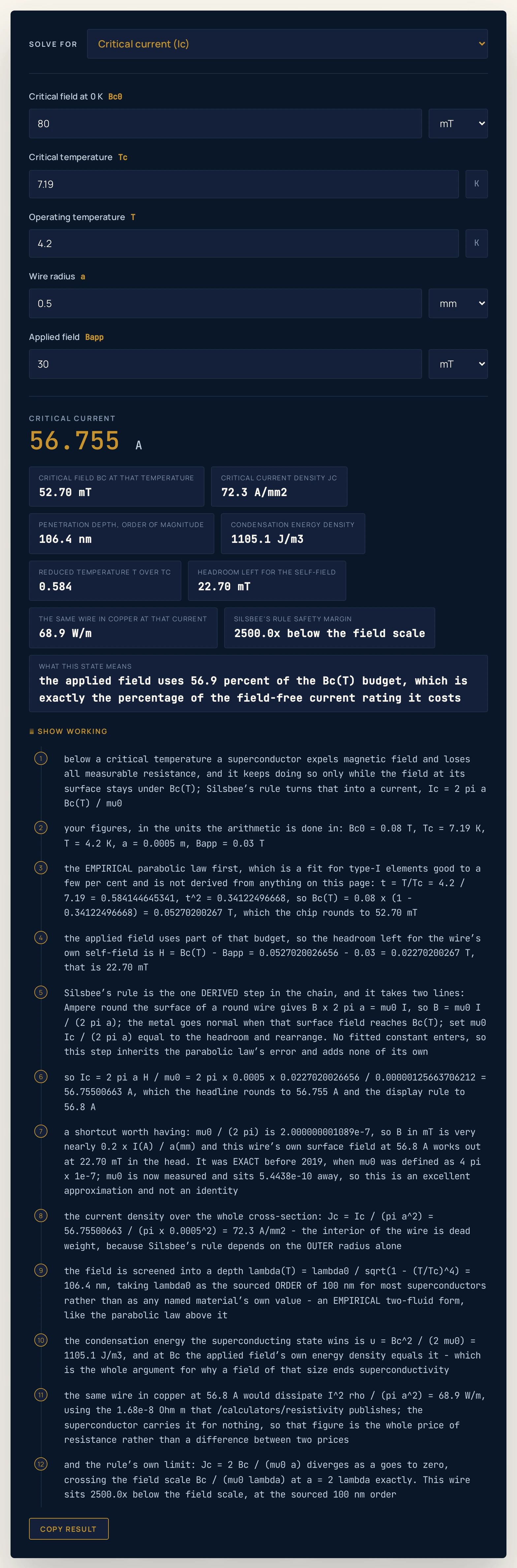
52.70 mT because the temperature has not moved, but the headroom is down to 22.70 mT and the answer has collapsed to 56.755 A — the worded chip gives the arithmetic as 56.9 per cent of the budget spent.Where the superconductor calculator breaks down
The arithmetic is exact to the last digit a double can hold. What fails is an empirical fit being quoted as if it were a law, a type-I model being asked about a type-II magnet, a sub-micron wire being described by a rule that assumes a surface, or a diameter being typed where a radius belongs.
- The critical-field law is an empirical fit, not a derivation
- Everything in the banner rests on
Bc(T) = Bc0[1 − (T/Tc)2], which is the standard fit for type-I elements and is good to a few per cent rather than exactly. Nothing on this site derives it, and this page does not pretend otherwise. Silsbee’s rule on top of it is exact given the field, so the answer carries the fit’s error and no more — which also means a result quoted to six figures is precise rather than accurate. - Silsbee’s rule contains its own failure, at a radius you can name
- The critical current density
Jc = 2Bc/(μ0a)grows without limit as the wire gets thinner, which cannot be physics. It crosses the field scaleBc/(μ0λ)ata = 2λexactly, with no coefficient and independently of material, field and temperature. Taking the sourced 100 nm order forλ, a 1 mm-diameter wire sits 2500 times below that scale, a 0.2 mm magnet wire 500 times, a 5 µm-diameter filament of the sort real cable is made from only 12.5 times, a 400 nm nanowire exactly at it, and a 100 nm nanowire 4 times over it. The safety-margin chip for Silsbee’s rule prints which of those you are in. - No named material is given a penetration depth here
- This cluster sourced an order of magnitude and not a table: 100 nm is the published figure for “most superconductors”, and the chip says order of magnitude for that reason. Nothing on this page gives lead, tin, mercury or any other element its own
λ, its coherence length, its carrier density, its molar mass or its low-temperature heat capacity, because none of those was sourced. Treat every penetration-depth figure here as an order and nothing finer. - The penetration depth diverges at the critical temperature
- Silsbee’s rule quietly assumes the current hugs a surface, and
λ(T) = λ0/sqrt(1 − (T/Tc)4)— also an empirical form — runs away as the critical temperature is approached, so that assumption must fail somewhere. Solvingλ(T*) = aputs the failure absurdly close toTc: for a 0.500 mm lead wire the window is 71.9 nanokelvin wide. For a 2.5 µm-radius filament it is 2.8777 mK, about forty thousand times wider, and that is the direction that matters. - Type-II materials are a different quantity and no formula here touches them
- Real magnets are wound from type-II material, which above a first critical field admits magnetic flux as quantised vortices and stays superconducting up to a much higher upper critical field. That upper field is not the type-I thermodynamic critical field this page computes, so neither the parabolic law nor Silsbee’s rule may be applied to the rows below. They are printed as context only.
- Only the outer radius enters, so the tool cannot describe a real conductor
- Silsbee’s rule takes no wall thickness and no filament count, which is exactly why the tube result works — but it also means this page cannot tell you whether a given wall is thick enough, whether a filament array is stable, or what the copper matrix around it is doing. A wall of one penetration depth would be 0.0399960 per cent of the metal and is below the
2λscale above, so it is not a safe design and nothing here should be read as saying it is. - A round, isolated wire in a uniform field, and nothing else
- The geometry is a single straight round wire with a uniform applied field, and a real magnet is a wound coil whose own turns add field to each other. There is no flux jump, no thermal runaway, no ac loss, no strain dependence and no mechanical force in this model, and all four of those decide whether a real magnet works. Nothing here is a measurement of any apparatus.
- Two zeros are answers and one demand is a refusal
- At or above the critical temperature, and with an applied field at or above the critical field, the critical current is exactly zero — a physical answer, printed as
0, with the worded chip saying which of the two it is. The refusal is different in kind: a demanded current above the critical current at absolute zero has no solution at any temperature, so the operating-temperature mode declines rather than answering 0 K. For a 0.500 mm lead wire that ceiling is 199.999999891 A, which is why 200.1 A is refused. - Do not re-derive one printed figure from another
- Every chip is rounded on its own before it is printed, and the calculation behind it is not. At 4.2 K the critical field chip reads
52.70 mTwhere the exact value is 52.702003 mT, and putting the printed figure back through Silsbee’s rule gives 131.750 A against the 131.755 A the exact chain gives, a gap of 0.005007 A. Every chip on this page is computed from the exact values and rounded once, which is the only way the arithmetic stays self-consistent; Show working prints the unrounded value so the rounding is visible. - The condensation-energy figure in the text is a one-sided bound
- The 1.754 mK warming quoted above uses lead’s room-temperature specific heat, which is the only figure this site publishes for it. Heat capacity falls steeply on cooling, so the real temperature rise at 4 K is larger than that — the statement is “at least 1.754 mK” and never “1.754 mK”. No low-temperature heat capacity was sourced for any material in this cluster, and none is given.
- Nothing here is about room-temperature superconductivity
- The highest critical temperature on this page is the 95 K of the YBCO row in the context table, and that row is context rather than something the formulas describe. No claim of any kind is made about superconductivity at or near room temperature, because nothing was sourced for it.
- The calculator measures nothing — you supply every figure
- Five numbers go in, one relation is rearranged, and the answer describes that idealised wire and nothing else. The preset names are shorthand for the figures beside them rather than claims about any apparatus, and the material values are a retrieved table rather than a measurement made here. Verify anything you mean to rely on against your own data before you quote it.
| Material | Critical temperature / K | Upper critical field / T |
|---|---|---|
| Niobium (Nb) | 9.26 | 0.82 |
| Niobium-titanium (NbTi) | 10 | 15 |
| Niobium-tin (Nb3Sn) | 18.3 | 30 |
| Magnesium diboride (MgB2) | 39 | 74 |
| YBCO cuprate | 95 | 120 to 250 (a range) |
Where zero resistance is actually used
- Magnet coils, and why they are not wound from a type-I metal
- A magnet is the obvious use of a wire that carries current for nothing, and the arithmetic on this page explains at once why lead is not the wire for it. The energy density of a 1 T field is 156.25 times lead’s entire condensation energy at absolute zero, so the field would destroy the state long before the magnet was useful. Medical scanner magnets are wound from type-II material instead, and those coils are already described in the guide to electromagnets; type-II material is outside this calculator’s model entirely.
- Why real cable is filaments rather than rods
- The critical current depends on the outer radius alone, so the interior of a thick rod contributes nothing and a tube of the same outer radius matches it on a fraction of the metal. Real superconducting cable takes that to its conclusion: thousands of filaments a few microns across, embedded in a normal-metal matrix. Run the 0.0500 mm row and the 0.500 mm row together and the trade is visible — a tenth of the current at ten times the current density.
- Persistent currents, and the measurement that bounds the resistance
- Start a current going round a closed superconducting loop and there is no obvious reason for it to stop, which is the claim this topic is famous for. The sourced record is 10467 days in a gravimeter coil in Belgium; combined with a stated coil inductance and a stated detection floor, that puts an upper bound on the loop’s resistance rather than proving it is zero. The electric current calculator turns such a current into a charge per second, and the resistance simulator shows what the same wire does when it is an ordinary metal instead.
- Cryogenics: what temperature the whole subject needs
- Every type-I element in the table above needs liquid helium, which boils at 4.22 K, and the opening case is set at 4.2 K for that reason. Liquid nitrogen at 77.36 K is far cheaper and far easier, and on the sourced numbers exactly one row of the type-II context table — the 95 K cuprate — can be cooled with it. That single fact is the whole reason the cuprates mattered.
- The lecture demonstration everyone has seen
- A small magnet floating above a cooled disc is the image most people have of superconductivity, and it is a real effect. Its physics is flux pinning in a type-II material, which is a different mechanism from the field expulsion this calculator models, so no number on this page describes it. It is a demonstration worth watching and not a measurement to put a figure on.
- Counting what resistance costs
- The copper chip is the point of comparison the whole topic needs. A 1 mm-diameter copper wire has a resistance of 0.0213904 Ω per metre, so carrying the lead wire’s 131.755 A costs
371.3 W/m— roughly a hot plate for every metre of cable. Because the current goes as the radius and the resistance per metre as its inverse square, that figure is unchanged at 371.3 W/m for the 1.000 mm wire as well, which is an exact lockstep rather than a coincidence.
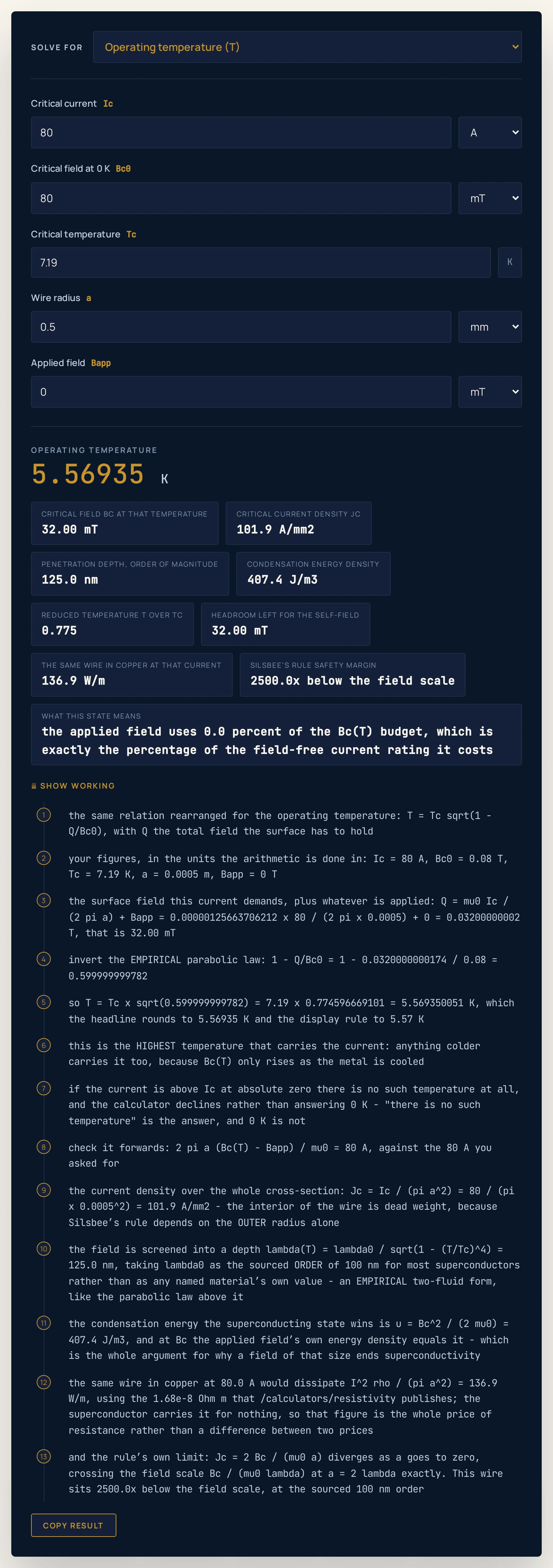
5.56935 K — comfortably above liquid helium’s 4.22 K, so this one is buildable.Where to go next
For the definition, the derivation in full, the drawn phase diagram and eight worked problems, read the guide to superconductors, which this tool is the arithmetic half of. The guide to electrical resistance is the piece it answers: it promises the persistent-current result and leaves the numbers to this page.
Three more are worth a bookmark. The resistivity calculator is where the copper figure used here comes from; the magnetic field calculator handles the field inside a coil rather than at a wire’s surface; and the absolute zero calculator converts the temperatures this whole subject is quoted in. The full physics lab library and the calculator index are open too.
Frequently asked questions
What does the superconductor calculator work out?
It works out how much current a superconducting wire can carry before it goes back to being an ordinary resistive metal. Enter the critical field at absolute zero, the critical temperature, the temperature you are holding the wire at, its radius and any applied field, and it returns the critical current from Silsbee's rule, Ic = 2 pi a times the field headroom divided by mu nought. Point the Solve for menu at the radius, the critical field, the operating temperature or the critical temperature instead and it rearranges the same relation, so a demanded current can give you back the temperature you need to reach.
What is a superconductor?
A superconductor is a material that below a certain temperature loses all measurable electrical resistance and expels magnetic field from its interior. The temperature is called the critical temperature, and the expulsion of field is the Meissner effect. Both properties end together: raise the temperature, the current or the surrounding field far enough and the material returns to being an ordinary metal, which is the boundary this calculator computes.
Why does a superconductor have a maximum current at all, if its resistance is zero?
Because a current makes a magnetic field, and a superconductor can only hold out a limited field. Ampère's law says the field at the surface of a round wire is mu nought times the current divided by two pi times the radius, so pushing more current through raises the field at its own surface. When that self-field reaches the critical field the material can no longer expel it and goes normal. That argument is Silsbee's rule, and it takes two lines with no fitted constant in it.
Is the critical field formula exact?
No, and the distinction matters. The parabolic law, which says the critical field falls as one minus the square of the temperature divided by the critical temperature, is an empirical fit: it describes type-I elements to a few per cent and is not derived from anything. Silsbee's rule, which turns that field into a current, is exact given the field, so it inherits the fit error and adds none of its own. The working on this page labels which step is which.
Why does the answer go up when I make the wire thicker, but the current density goes down?
Because the critical current depends on the circumference and not on the area. Doubling the radius doubles the critical current while quadrupling the cross-section, so the current density halves. That is why the inside of a superconducting wire is dead weight and why real superconducting cable is thousands of fine filaments in a copper matrix rather than one thick rod. For copper the contrast holds only against the fixed current density rule of thumb: at a fixed limit in watts per metre, copper ampacity also scales with the radius.
Why is 0 A an answer here rather than an error?
Because it is the physically correct answer in two cases. If the operating temperature is at or above the critical temperature the metal is a normal conductor, and if the applied field alone is at or above the critical field at that temperature the wire is already quenched before any transport current flows. Both give a critical current of exactly zero, and the worded chip says which of the two it is. The one genuine refusal is a demanded current above the critical current at absolute zero, where no temperature works at all and zero kelvin is not the answer.
Why do the numbers on the page not quite reproduce each other by hand?
Because every chip is rounded on its own before it is printed, and the calculation behind it is not. At 4.2 K lead has a critical field of 52.702003 millitesla, which prints as 52.70; re-deriving the current from that printed figure gives 131.750 A where the exact chain gives the 131.755 A the headline shows. The gap is only 0.005007 A, but it is real, and the Show working panel prints the unrounded value on purpose so the rounding is visible rather than assumed.
Can I use this for niobium-titanium or for a high-temperature superconductor?
No, and the reason is that they are a different kind of superconductor. Niobium-titanium, niobium-tin, magnesium diboride and the cuprates are type-II materials: above a first critical field they let magnetic flux in as quantised vortices and stay superconducting up to a much higher upper critical field, so neither the parabolic law used here nor Silsbee's rule describes them. This page models a type-I element, and the type-II table on it is context only, with no formula applied to any of its rows.
What does zero resistance actually save?
At the opening figures, a 1 mm-diameter lead wire at 4.2 K carries 131.755 A for nothing. The same wire in copper, using the 1.68e-8 ohm metre this site publishes, has a resistance of 0.0213904 ohms per metre and burns 371.3 W per metre of cable carrying that current. That is roughly a hot plate for every metre, and it is the whole price of resistance rather than a difference between two prices, because the superconductor dissipates nothing at all.
References & formula source
- Bc(T) = Bc0[1 - (T/Tc)^2] is the parabolic critical-field law, the standard EMPIRICAL fit for type-I elements and good to a few per cent. It is not derived on this page, and no page in this cluster derives it: two endpoints and a monotonic fall between them are all it claims.
- Ic = 2 pi a Bc(T) / mu0 is Silsbee's rule, and it IS derived, in two lines. Ampère's law round the surface of a round wire gives B times 2 pi a = mu0 I; the material goes normal when the field at its surface reaches Bc(T); equate the two and rearrange. No fitted constant enters, so the step is exact given the parabolic law.
- lambda(T) = lambda0 / sqrt(1 - (T/Tc)^4) is the two-fluid temperature dependence of the London penetration depth, EMPIRICAL on the same footing as the parabolic law. lambda0 is taken as 100 nm throughout, which is the published ORDER OF MAGNITUDE for most superconductors and is never presented as any named material's own value.
- Critical temperatures and critical fields for the eleven type-I elements, and the critical temperatures and UPPER critical fields for the five type-II materials in the context table, are from the Wikipedia list of superconductors, retrieved 2026-09-27. YBCO is given a range of 120 to 250 T there rather than a single figure, and it is quoted as a range here for that reason.
- mu0 = 1.25663706212e-6 N/A^2 is the CODATA 2018 value, and it has been a MEASURED quantity rather than an exact one since the 2019 redefinition of the SI. That is why mu0 divided by two pi is 2.000000001089e-7 rather than exactly 2e-7, and why the convenient shortcut B in millitesla equals 0.2 times the current in amps divided by the radius in millimetres is an excellent approximation and not an identity.
- rho = 1.68e-8 Ohm m for copper is the figure /calculators/resistivity already publishes on this site, and it is the only resistivity used anywhere on this page. No other material is given a resistivity here.
- The 10467-day persistent current quoted in the text is the superconducting gravimeter record from 4 August 1995 to 31 March 2024, reported on the Wikipedia superconductivity article. The coil inductance and the detection floor combined with it to give a resistance bound are STATED ASSUMPTIONS rather than measurements, and the result is a bound and not a proof that a persistent current cannot decay.
- Every figure quoted in the text above is a string this calculator printed for the inputs named beside it, a constant the page states, or a ratio the cluster's independent reference asserts. No figure on this page was worked out by hand.
- Further reading: Superconductivity — Wikipedia