The eddy currents simulator draws 100 cm3 of non-magnetic metal end-on in an alternating field, with the induced loops circulating inside it, and slices that same block into as many as forty insulated laminations while you watch. A second band underneath plots how far the current actually reaches across the metal, with the skin depth marked on it. Four sliders set the field, the frequency, the number of slices and the resistivity; eleven readouts answer — ten numbers and a status sentence — including the one pair this lab exists for: the cut you really get beside the cut the d2 rule promises.
Eddy Currents: Why a Core Is Sliced Up
A block of non-magnetic metal (μr = 1) sits in an alternating field that runs along it, into the page. The changing flux drives loops of current inside the solid metal — eddy currents — and they turn real power into heat. Cut the same 100 cm3 of metal into N insulated laminations and the loops shrink with the slices. The gold card is the exact slab solution; the blue card is the textbook estimate π2B2f2d2 / 6ρ, which assumes the field reaches the middle of the metal. The second band shows whether it does.
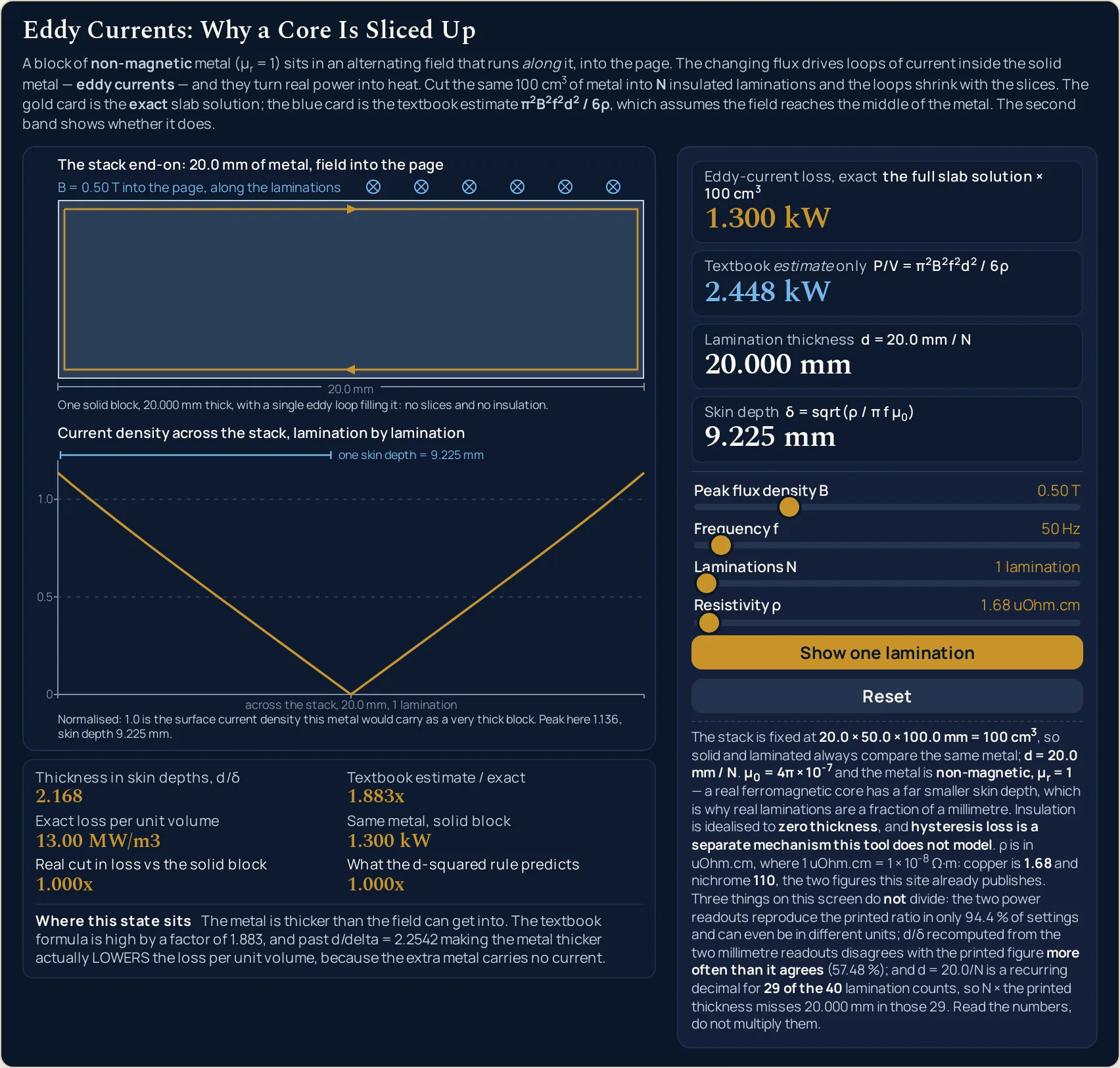
Thickness in skin depths, d/δ2.168
Textbook estimate / exact1.883x
Exact loss per unit volume13.00 MW/m3
Same metal, solid block1.300 kW
Real cut in loss vs the solid block1.000x
What the d-squared rule predicts1.000x
Where this state sitsThe metal is thicker than the field can get into. The textbook formula is high by a factor of 1.883, and past d/delta = 2.2542 making the metal thicker actually LOWERS the loss per unit volume, because the extra metal carries no current.
Eddy-current loss, exact the full slab solution × 100 cm3
1.300 kW
Textbook estimate only P/V = π2B2f2d2 / 6ρ
2.448 kW
Lamination thickness d = 20.0 mm / N
20.000 mm
Skin depth δ = sqrt(ρ / π f μ0)
9.225 mm
Peak flux density B0.50 T
Frequency f50 Hz
Laminations N1 lamination
Resistivity ρ1.68 uOhm.cm
The stack is fixed at 20.0 × 50.0 × 100.0 mm = 100 cm3, so solid and laminated always compare the same metal; d = 20.0 mm / N. μ0 = 4π × 10-7 and the metal is non-magnetic, μr = 1 — a real ferromagnetic core has a far smaller skin depth, which is why real laminations are a fraction of a millimetre. Insulation is idealised to zero thickness, and hysteresis loss is a separate mechanism this tool does not model. ρ is in uOhm.cm, where 1 uOhm.cm = 1 × 10⁻⁸ Ω·m: copper is 1.68 and nichrome 110, the two figures this site already publishes.
Three things on this screen do not divide: the two power readouts reproduce the printed ratio in only 94.4 % of settings and can even be in different units; d/δ recomputed from the two millimetre readouts disagrees with the printed figure more often than it agrees (57.48 %); and d = 20.0/N is a recurring decimal for 29 of the 40 lamination counts, so N × the printed thickness misses 20.000 mm in those 29. Read the numbers, do not multiply them.
Three things on this screen do not divide: the two power readouts reproduce the printed ratio in only 94.4 % of settings and can even be in different units; d/δ recomputed from the two millimetre readouts disagrees with the printed figure more often than it agrees (57.48 %); and d = 20.0/N is a recurring decimal for 29 of the 40 lamination counts, so N × the printed thickness misses 20.000 mm in those 29. Read the numbers, do not multiply them.
Load a real core on the sliders
Each button presses the lab’s own Reset first, which also returns the canvas to the whole-stack view, and then writes all four sliders, so a load never inherits where the last one left off. Work down the list in order: the first three cut the same copper finer and finer, and the last two change the frequency and the metal instead.
Pick a case above, or drag the four sliders yourself.
What Is the Eddy Currents Simulator?
The eddy currents simulator is a free interactive physics lab that runs in your browser, with nothing to install and no sign-up. It draws a fixed 100 cm3 stack of non-magnetic metal end-on in an alternating field — 20.0 mm thick, with the field running along the laminations and into the plane of the drawing — and circulates an eddy-current loop inside every slice the stack is divided into. A second band beneath plots the current density across the metal on a fixed normalised scale, with one skin depth marked on it, so the screening that makes the textbook formula fail is visible rather than merely stated.
Four sliders set the peak flux density from 0.05 to 2.00 T, the frequency from 10 to 1000 Hz, the number of insulated laminations from 1 to 40 and the resistivity from 1.00 to 120.00 uOhm.cm.
Four cards answer with the exact eddy-current loss in the stack, the textbook estimate P/V = π2B2f2d2 / (6ρ) on its own, the thickness of one lamination and the skin depth δ = sqrt(ρ / (π f μ0)). Six smaller cells give the thickness in skin depths, the ratio of estimate to exact, the loss per unit volume, the loss the same metal would have uncut, and the headline pair: the cut in loss the metal really delivers beside the cut the d2 rule predicts.
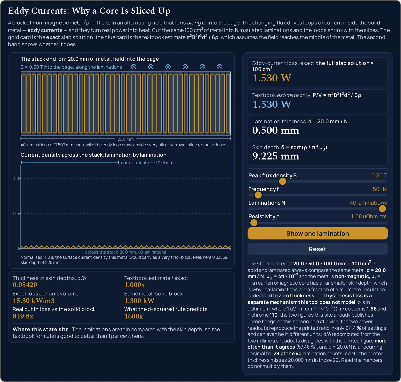
That pair is what the lab is for. Cutting the same copper into forty 0.500 mm slices takes the loss from 1.300 kW to 1.530 W, a real cut of 849.8 times where the rule promises 1600 — because the rule was overstating the solid block by 1.883 before any cutting happened. A wrapping status line names the regime the current state sits in and says whether the estimate may be quoted at all, and a Show one lamination button magnifies the profile band to a single slice without changing a single reading. The metal is non-magnetic, with a relative permeability of one, so hysteresis is not modelled and no figure is offered for electrical steel.
| Control | Range | Step |
|---|---|---|
| Peak flux density | 0.05 to 2.00 T | 0.05 T |
| Frequency | 10 to 1000 Hz | 10 Hz |
| Laminations | 1 to 40 | 1 |
| Resistivity | 1.00 to 120.00 uOhm.cm | 0.02 uOhm.cm |
How to use the eddy currents simulator
- Start from the state it opens in. The sliders read Peak flux density B 0.50 T, Frequency f 50 Hz, Laminations N 1 lamination and Resistivity ρ 1.68 uOhm.cm, and the four cards answer 1.300 kW, 2.448 kW, 20.000 mm and 9.225 mm. Reset returns all four sliders to that and replays the loops growing in.
- Drag Laminations N and watch the loops, not the number. It runs from 1 to 40 in steps of 1. Each slice gets its own loop and the loops shrink with the slices, while Eddy-current loss, exact falls from 1.300 kW to 24.48 W at ten and 1.530 W at forty. The quantity of metal never changes.
- Read the headline pair at the bottom of the grid. Real cut in loss vs the solid block and What the d-squared rule predicts sit side by side on purpose. At forty laminations they read 849.8x and 1600x, and that gap is the most useful thing on the panel.
- Watch the two power cards converge. Uncut, Textbook estimate only reads 2.448 kW against the exact card’s 1.300 kW. By ten laminations both read 24.48 W and by forty both read 1.530 W. The estimate is not wrong everywhere — it is wrong where the metal is thick.
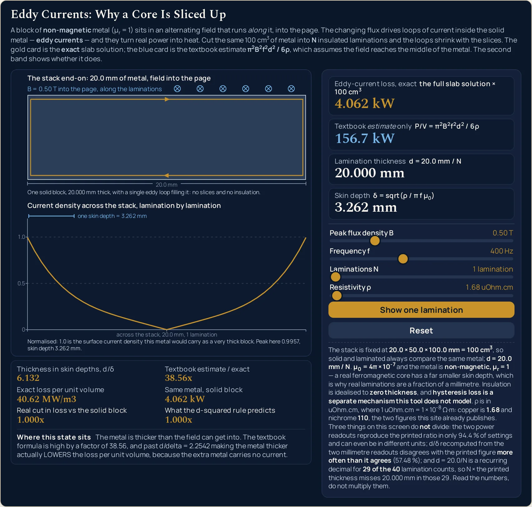
- Move Frequency f and watch the skin depth first. It runs from 10 to 1000 Hz in steps of 10, and the Skin depth card falls as it climbs: 9.225 mm at 50 Hz, 3.262 mm at 400 Hz and 2.063 mm at the 1000 Hz top stop, all three in copper.
- Move Resistivity ρ. It runs from 1.00 to 120.00 uOhm.cm in steps of 0.02, and only two positions on it are named metals here: 1.68 is copper and 110.00 is nichrome. The second loses 37.38 W uncut where copper loses 1.300 kW.
- Move Peak flux density B and notice what stays still. It runs from 0.05 to 2.00 T in steps of 0.05. Every power on the panel moves with it; the thickness, the skin depth, the thickness in skin depths, the ratio of estimate to exact, the real cut and the predicted cut all stay exactly where they are, because none of them contains the field.
- Press Show one lamination. The button relabels itself Show the whole stack, the lower band magnifies to a single slice and its heading and horizontal axis are rewritten. Not one readout changes, which is the point: the view is a magnifying glass, not a different calculation.
- Read the status line last. Where this state sits names the regime in a full sentence and tells you whether the textbook card may be quoted at all. It is the readout to check before you copy any figure off this panel into anything else.
The step worth repeating is the second one. Take Laminations N from 1 to 40 slowly and watch three things move together: the slices narrow, the loops inside them shrink, and the lower band’s one near-straight V flattens into a shallow ramp inside every slice — forty of them by the top of the slider. The shape that crowds all its current into the two faces and empties the middle belongs to Four hundred hertz, not to this state. The loss card is only reporting what the drawing already showed you.
Which way the loops turn is settled by Lenz’s law rather than by anything on this panel, and it is the one thing this lab draws without explaining: each loop flows the way that opposes the change that created it. The guide to Lenz’s law makes that argument properly, and the Lenz’s law simulator shows the same opposition in a coil, where there is a wire to follow.
Worked example: change one thing at a time
Every row below is one setting of the four sliders, and every cell is a string the running lab printed there. The first, fourth, fifth, seventh and ninth rows are on the preset buttons above; the rest are a drag away. Where a cell and the lab ever part company, believe the lab.
| Setting | Sliders, as the panel reads them | Eddy-current loss, exact | Textbook estimate only | Skin depth | Thickness in skin depths | Estimate over exact |
|---|---|---|---|---|---|---|
| Solid copper block | 0.50 T · 50 Hz · 1 lamination · 1.68 uOhm.cm | 1.300 kW | 2.448 kW | 9.225 mm | 2.168 | 1.883x |
| Two laminations | 0.50 T · 50 Hz · 2 laminations · 1.68 uOhm.cm | 579.6 W | 612.0 W | 9.225 mm | 1.084 | 1.056x |
| Four laminations | 0.50 T · 50 Hz · 4 laminations · 1.68 uOhm.cm | 152.5 W | 153.0 W | 9.225 mm | 0.5420 | 1.003x |
| Cut it into ten | 0.50 T · 50 Hz · 10 laminations · 1.68 uOhm.cm | 24.48 W | 24.48 W | 9.225 mm | 0.2168 | 1.000x |
| Cut it into forty | 0.50 T · 50 Hz · 40 laminations · 1.68 uOhm.cm | 1.530 W | 1.530 W | 9.225 mm | 0.05420 | 1.000x |
| Double the field | 1.00 T · 50 Hz · 1 lamination · 1.68 uOhm.cm | 5.200 kW | 9.791 kW | 9.225 mm | 2.168 | 1.883x |
| Four hundred hertz | 0.50 T · 400 Hz · 1 lamination · 1.68 uOhm.cm | 4.062 kW | 156.7 kW | 3.262 mm | 6.132 | 38.56x |
| Four hundred hertz, cut | 0.50 T · 400 Hz · 40 laminations · 1.68 uOhm.cm | 97.91 W | 97.91 W | 3.262 mm | 0.1533 | 1.000x |
| A more resistive metal | 0.50 T · 50 Hz · 1 lamination · 110.00 uOhm.cm | 37.38 W | 37.38 W | 74.650 mm | 0.2679 | 1.000x |
| The resistive metal cut | 0.50 T · 50 Hz · 40 laminations · 110.00 uOhm.cm | 23.37 mW | 23.37 mW | 74.650 mm | 0.006698 | 1.000x |
| The most screened state | 2.00 T · 1000 Hz · 1 lamination · 1.00 uOhm.cm | 79.58 kW | 26.32 MW | 1.592 mm | 12.57 | 330.7x |
| The gentlest state | 0.05 T · 10 Hz · 40 laminations · 120.00 uOhm.cm | 8.567 uW | 8.567 uW | 174.346 mm | 0.002868 | 1.000x |
Rows 1 to 5 are the lab in one column. Nothing changes down them except how the same copper is divided, and the loss runs 1.300 kW, 579.6 W, 152.5 W, 24.48 W, 1.530 W. Watch the last column at the same time: it starts at 1.883x and is at 1.000x by the fourth row, so the textbook estimate becomes trustworthy exactly as the slices become thin.
Rows 6 and 7 are the two ways to make it worse. Doubling the field doubles neither power card — it quadruples both, 1.300 kW to 5.200 kW, which is the squared field in both formulas restated rather than anything the lab found. What is worth watching is that every other readout stays exactly where it was. Raising the frequency to 400 Hz does something different: the skin depth drops to 3.262 mm, the estimate climbs to 156.7 kW and the metal delivers 4.062 kW, so the estimate is now 38.56x too big.
Rows 9 and 10 change the metal rather than the geometry. Nichrome uncut loses 37.38 W where copper uncut loses 1.300 kW, and its skin depth of 74.650 mm is nearly four times the whole block, so its estimate is exact in both rows. The resistivity slider is the one control that improves the answer and the validity together. Where that 1.68 comes from is the resistivity calculator, which publishes both metals.
Rows 11 and 12 are the two ends of what this grid can do. The most screened state it reaches prints 79.58 kW beside an estimate of 26.32 MW — out by 330.7x, the largest overshoot here — and the gentlest prints 8.567 uW. Nearly ten orders of magnitude separate those two, which is why the power cards carry a unit switch rather than a fixed unit.
Neither of them is the biggest loss, though, and that is worth finding by hand. Set 2.00 T, 1000 Hz and copper, then walk Laminations N up from 1: the loss climbs from 103.2 kW uncut to 413.2 kW at four laminations before it starts to fall. The real cut card reads 0.2497x there — cutting the block made it four times worse.
| Laminations | Lamination thickness | Eddy-current loss, exact | Real cut in loss vs the solid block | What the d-squared rule predicts |
|---|---|---|---|---|
| 1 lamination | 20.000 mm | 1.300 kW | 1.000x | 1.000x |
| 2 laminations | 10.000 mm | 579.6 W | 2.243x | 4.000x |
| 4 laminations | 5.000 mm | 152.5 W | 8.528x | 16.00x |
| 10 laminations | 2.000 mm | 24.48 W | 53.12x | 100.0x |
| 40 laminations | 0.500 mm | 1.530 W | 849.8x | 1600x |
That table is the reason this lab exists. The two right-hand columns leave the first row together and end forty laminations later at 849.8x against 1600x. The shortfall is a factor of 1.8828, and lamination still works — it works nearly as well as advertised, but not quite, and the gap has a single cause.
That cause is the first row, not the last. The d2 rule compares every cut against a solid block whose loss it had already overstated by 1.883, so the promised 1600-fold cut was measured from a number the metal never had. Read the exact column instead and the cut is honest at every count.
Formula and symbol reference
Two relations drive the whole panel. The textbook estimate is the classical thin-sheet loss, P/V = π2B2f2d2 / (6ρ), and the validity test beside it is the skin depth, δ = sqrt(ρ / (π f μ0)). The exact card solves the same slab without the thin-sheet assumption, which is why the two cards agree at forty laminations and part company at one.
The cards themselves print those two lines without the inner brackets, as / 6ρ and sqrt(ρ / π f μ0), which is how they are read aloud and how the code evaluates them. The brackets are written in here because a divide followed by a product is ambiguous on a page in a way it is not in speech, and the figures the lab prints are the bracketed reading.
| Symbol | Meaning | SI unit | In this lab |
|---|---|---|---|
| B | Peak flux density of the alternating field, set by the Peak flux density B slider. It runs along the laminations, into the plane of the drawing, and the loss goes as the square of it | tesla, T | 0.05 to 2.00 in steps of 0.05, printed to two decimals: “0.50 T” after Reset, “2.00 T” at the top stop. Doubling it to 1.00 T takes the loss from 1.300 kW to 5.200 kW and moves nothing else on the panel. |
| f | Frequency of the field, set by the Frequency f slider. It does two jobs at once: it raises the loss and it shrinks the skin depth, which is what makes the top of this slider interesting | hertz, Hz | 10 to 1000 in steps of 10, printed as a whole number: “50 Hz” after Reset, “400 Hz” on the aircraft case and “1000 Hz” at the top stop, where copper’s skin depth is down to 2.063 mm. |
| N | Number of insulated laminations the 20.0 mm stack is divided into, set by the Laminations N slider. The quantity of metal never changes — only how it is cut | dimensionless count | 1 to 40 in steps of 1, printed with its own noun: “1 lamination” after Reset and “40 laminations” at the top stop. |
| ρ | Resistivity of the metal, set by the Resistivity ρ slider. A more resistive metal carries a smaller eddy current for the same induced field, and it also lets the field reach further in | ohm metre, Ω m (the slider is in microhm-centimetres) | 1.00 to 120.00 in steps of 0.02, printed to two decimals: “1.68 uOhm.cm” is copper and “110.00 uOhm.cm” is nichrome. Those are the only two values this lab names as a material; every other position is a metal you are positing. |
| d | Thickness of ONE lamination, printed by the Lamination thickness card and never typed. It is the stack divided by the count, and it is the quantity the whole topic turns on | metre, m (the card is in millimetres) | three decimals in millimetres: “20.000 mm” uncut, “2.000 mm” at ten and “0.500 mm” at forty. It is a recurring decimal at most counts, so the card rounds it. |
| δ | Skin depth, printed by the Skin depth card. The distance the alternating field reaches into this metal, and the yardstick the thickness has to be measured against | metre, m (the card is in millimetres) | three decimals in millimetres, and it depends on the metal and the frequency only: “9.225 mm” for copper at 50 Hz, “3.262 mm” at 400 Hz, “74.650 mm” for nichrome at 50 Hz and “174.346 mm” at the gentlest corner of the sliders. |
| d/δ | Thickness in skin depths, printed by the Thickness in skin depths cell. The single number that decides whether the textbook estimate may be quoted | dimensionless | four significant figures: “2.168” for the solid copper block, “0.05420” at forty laminations, “6.132” at 400 Hz uncut and “12.57” at the worst corner, which is the largest this grid reaches. |
| P | Eddy-current loss in the whole 100 cm3 stack, printed by the Eddy-current loss, exact card from the unapproximated slab solution | watt, W | four significant figures with a uW, mW, W, kW or MW switch chosen after the rounding: “1.300 kW” uncut, “1.530 W” at forty and “8.567 uW” at the gentlest corner, which is the smallest this lab reaches. |
| P/V | The same loss per unit volume, printed by the Exact loss per unit volume cell. It is the density rather than the total, so it is what you would compare against another block of a different size | watt per cubic metre | four significant figures with the same unit ladder: “13.00 MW/m3” uncut, “15.30 kW/m3” at forty and “795.8 MW/m3” at the worst corner. |
| μ0 | Permeability of free space, the one constant typed into this lab. The metal is taken to be non-magnetic, so its own permeability is this same value | henry per metre, H/m | a constant: 4π × 10−7 H/m. The SI 2019 figure 1.25663706212e-6 is larger by about 5.4 parts in ten thousand million and gives the same 9.225 mm skin depth here. |
Two rows there are not sliders. The lamination thickness and the skin depth are both computed and printed rather than typed, and they are the pair whose ratio the whole page turns on. If the resistivity is the unfamiliar quantity of the four, the guide to electrical resistance covers what it means before it gets anywhere near a magnetic field.
The physics: what the two bands are for
The upper band answers the question the topic is named after. Put metal in a changing field and the induced electric field drives current round closed paths inside the metal itself, with nothing to guide it; cut the metal into insulated slices and those paths can no longer cross the cuts, so each slice gets a loop of its own. The drawing shows the loops shrinking in both directions at once, which is where the square comes from.
The lower band answers the question that makes the loss card disagree with the estimate card. It plots the current density across the metal against a scale on which 1.0 is what the surface of a very thick block would carry, and the caption gives the peak. Uncut copper at mains peaks at 1.136; the same copper in forty slices peaks at 0.03832, because a thin slice never gets near the surface value anywhere.
Now load Four hundred hertz and look at the lower band alone. The near-straight V of the 50 Hz block has become a deep rounded valley: the peak is 0.9957 at each face, the middle sinks to nothing and stays there across most of the span, and the ruler above marks one skin depth as 3.262 mm inside a 20 mm block. That shape is the whole of the overestimate — the textbook formula charges for current all the way across, and most of the way across there is none.
It also explains a result that sounds impossible. Past 2.2542 skin depths, making the metal thicker lowers the loss per unit volume, because the extra metal joins the dead zone rather than the conducting skin. The status line says so in words whenever you are past that line, and the Exact loss per unit volume cell is where you can watch it happen.
Read the status line and the ratio card together, never against each other. In the middle regime the sentence gives the overshoot as a percentage while Textbook estimate / exact gives it as a ratio: at two laminations the sentence says 5.583 per cent and the card says 1.056x. One is the other minus one, in per cent; neither divides into the other and 1.056x is not 1.056 per cent.
None of this touches the direction of the loops or the EMF that starts them, both of which belong upstream of this lab. The full guide to eddy currents carries the six-line derivation, the drawn geometry and eight worked problems, and the guide to electromagnetic induction sets out the induction all of it rests on.
d2 rule predicts. The profile band has collapsed from one tall curve to forty shallow ramps peaking at 0.03832.Where the eddy currents simulator breaks down
The lab solves its own model exactly, so nothing on the screen ever fails. Everything below is a limit of that model, of the slider grid, or of what a rounded display can carry, and each item says what this lab does about it.
- The metal is non-magnetic, with a relative permeability of one
- The skin depth here contains
μ0and no relative permeability, which is why a 20 mm block of copper can sit at only 2.168 skin depths at mains frequency. A real transformer core is a ferromagnetic alloy whose relative permeability runs into the thousands, so its skin depth is smaller by the square root of that factor — and that, rather than anything on this panel, is why real laminations are a fraction of a millimetre. No figure for any steel appears anywhere on this page, because none was measured for it. - Hysteresis is a separate loss and is not modelled at all
- A real magnetic core loses energy twice over: once to the currents this lab draws, and once to the work of turning the magnetisation round and back every cycle. That second loss rises roughly in proportion to the frequency where this one rises as its square, so it dominates at the low end, and a core loss quoted by a manufacturer normally contains both. There is no magnetisation to turn in a non-magnetic metal, so there is no such term here.
- The field is uniform, sinusoidal, and lies along the laminations
- One frequency, one amplitude, one direction, in the plane of the slices — which is what the strip above the stack is stating when it says the field runs into the page along the laminations. A square wave, a field with harmonics on it, a field that varies along the sheet or one with any component through the thickness all break the derivation. The Peak flux density B slider wants a peak rather than a root-mean-square value, and confusing the two changes the answer by a factor of two.
- The laminations are perfectly insulated and take up no room
- The insulation between slices is treated as having zero thickness, so the metal always fills the whole 20.0 mm and cutting it finer never costs any volume. A real stack has a stacking factor below one, has burrs at the cut edges that can short neighbouring sheets together, and has to find room for the varnish. All three push a real core above the figure on this panel.
- Each lamination is assumed wide and long compared with its thickness
- The model is one-dimensional: it solves across the thickness only, and treats the slice as unbounded in the other two directions. Real current has to turn round at the edges of a sheet, which adds path length the model knows nothing about, and the narrower the sheet the more that matters. The stack drawn here is 50 mm by 100 mm against slices as thin as 0.500 mm, which is comfortably inside the assumption but not infinitely so.
- The textbook card is an estimate, and its boundary is measured
- It is 0.5 per cent high at 0.5929 skin depths, 1 per cent at 0.7051, 5 per cent at 1.0545 and 10 per cent at 1.2542, and it keeps going: 1.883x for the uncut block at mains and 330.7x at the worst corner of these sliders. That is why the card is labelled an estimate and why the status line exists. The estimate is not a bad formula, either — it is a thin-sheet formula, and everything real that it is used on is thin.
- The two power cards do not divide to give the ratio cell
- Each is rounded to four significant figures on its own before you see it, and a ratio of two rounded numbers is not the rounded ratio. Dividing the printed strings fails to reproduce the printed Textbook estimate / exact figure in 5.60 per cent of a 60,000-state grid, and in some of those the two cards are not even in the same unit. Read the ratio cell, which is computed before any rounding happens.
- The thickness in skin depths does not recompute from the two millimetre cards either
- Both are rounded to three decimals in millimetres, and dividing one by the other disagrees with the printed Thickness in skin depths cell in 57.48 per cent of states — more often than it works. This is the trap that looks safest, because millimetres feel exact and three decimals feel generous. They are not; the cell is the figure to quote.
- The lamination thickness does not multiply back up to the stack
- The stack is 20.0 mm and the card shows
20.0/N, which is a recurring decimal for 29 of the 40 lamination counts — three slices give 6.667 mm on the card, and three times that is not 20.000. Multiplying the printed thickness by the count is not a check on anything. The stack thickness is fixed and stated; it is not a slider. - The status sentence and the ratio cell are one fact in two forms
- In the middle regime the sentence reports the overshoot as a percentage and the cell reports it as a ratio, so at two laminations you see 5.583 per cent and 1.056x on the same screen. They agree, and the arithmetic between them is subtraction rather than division. Quoting the ratio as a percentage, or the percentage as a ratio, is the one misreading this panel invites.
- The sliders stop where they stop, and the published figures stop with them
- The field runs 0.05 to 2.00 T, the frequency 10 to 1000 Hz, the count 1 to 40 and the resistivity 1.00 to 120.00 uOhm.cm. Every extreme quoted on this page — the 8.567 uW at the bottom, the 330.7x overshoot at the top, the 12.57 skin depths — is the most those four ranges can do, and a wider range would give different ones. The stack itself is fixed at 20.0 mm and cannot be moved at all.
- Nothing here has been measured
- Four slider positions go in and one idealised stack of metal comes out; no reading on this page describes a particular transformer, motor, hob or brake. Two resistivities are named as materials, copper and nichrome, and both are figures this site already publishes elsewhere. The difference between alternating and direct current is worth a look if the frequency slider is doing something you did not expect — at zero hertz there is no induction here at all, which is why the slider starts at ten.
Where eddy currents are actually used
- Choosing a lamination thickness against a loss budget
- This is the decision the sliders are shaped around. Set the field and the frequency your machine really runs at, then drag Laminations N until Eddy-current loss, exact lands under the waste heat you can afford to remove, and read the thickness off the card beside it. The answer is a design limit rather than a prediction, because everything the model leaves out pushes a real core the same way — upwards.
- Showing why faster equipment has to be laminated harder
- Press Four hundred hertz and then Solid copper block a few times. The same uncut metal goes from 1.300 kW to 4.062 kW, but the estimate card goes from 2.448 kW to 156.7 kW, so the naive scaling is wrong by more than the real change. Aircraft power runs at 400 Hz and switching supplies run far above it, which is why thickness stops being negotiable up there.
- Choosing the metal instead of the geometry
- The resistivity slider is the other lever, and it is the one most people expect to work backwards. Nichrome uncut loses 37.38 W where copper uncut loses 1.300 kW, because a more resistive metal carries a smaller current for the same induced EMF. It also pushes the skin depth out to 74.650 mm, which is why its estimate card is exact and copper’s is not.
- Teaching when a formula may be quoted at all
- Most tools print a number; this one prints a number and a sentence saying whether the number may be used. Dragging one slider until the status line changes its mind is a faster lesson in the validity of an approximation than any amount of small print, and it takes about four seconds. The habit it builds — check the regime before quoting the result — outlives the topic.
- Where the loss is wanted rather than avoided
- Induction heating, induction hobs and induction hardening all want exactly what a transformer designer is trying to remove, and the design goal flips: thick, reasonably resistive metal instead of thin slices, with the frequency chosen to put the skin depth where the heat is wanted. Set Laminations N to 1 and run the frequency up, and the lower band shows you the heat migrating to the surfaces as it goes.
- Braking and sensing without contact
- Anything that drags a conductor through a changing field gets a force for nothing and no parts to wear out, which is what eddy-current brakes on trains, the damping on a moving-coil needle and a magnet falling slowly down a copper pipe all have in common. Metal detectors and eddy-current crack testing read the same currents rather than fighting them. This lab does not compute any of those cases — it has one fixed geometry and no motion at all — but the currents it draws are theirs. What electricity costs to run is the other side of it for the cases where the heat is genuinely waste.
Where to go next
For the derivation in six lines, the drawn geometry and eight worked problems, read why metal cores are cut into slices. If you would rather type figures than drag them, and want six significant figures and the same relation run backwards for the field, the frequency, the thickness or the metal, the eddy current loss calculator is the first entry in the list below.
The neighbouring questions have tools of their own. Lenz’s law and its simulator settle which way the loops turn; electromagnetic induction and its lab own the EMF that starts them; and the Faraday’s law formula with its calculator handles the coil case rather than the solid one.
Further out, the guide to electrical resistance and the resistance lab cover the property the resistivity slider is setting, the guide to magnetic fields and the magnetic field lab cover the field before anything changes, and the guide to solenoids covers the coil that would be producing it. The rest is in the library of physics simulations and on the blog, and the site search will find a topic by name.
Frequently asked questions
Why does the textbook estimate card disagree with the exact loss card?
Because the textbook formula assumes the field reaches right through the metal, and past a certain thickness the eddy currents screen it out of the middle. Measured against the exact slab solution, it is good to 1 per cent while the lamination stays under 0.7051 skin depths and to 5 per cent out to 1.0545. At the worst state these sliders reach it is 330.7 times too big.
Why does cutting the block into forty slices not cut the loss 1600-fold?
Because the 1600 was never right about the block you started from. The panel prints 849.8x in the real cut card and 1600x in the card beside it, and the gap is the same 1.883 factor by which the textbook formula was already overstating the solid block at 2.168 skin depths. Cut the loss from a correct starting figure and the two agree.
The two power cards do not divide to give the ratio you print. Why not?
Your arithmetic is fine; the display is rounded. Each power is rounded to four significant figures on its own before you see it, and a ratio of two rounded numbers is not the rounded ratio. Over a 60,000-state grid the division fails to reproduce the printed ratio in 5.60 per cent of cases, and in some of those the two cards are not even in the same unit.
The status line says a percentage and the card says a ratio. Which is right?
Both, because they are one fact written two ways. At two laminations the card reads 1.056x and the sentence reads 5.583 per cent: the ratio is 1.05583, so the excess over one is 5.583 per cent. Read them together rather than against each other, and never quote 1.056x as a percentage.
Why does the skin depth not move when I drag the laminations slider?
Because the skin depth is a property of the metal and the frequency, not of how the metal has been cut. It is the square root of the resistivity divided by pi times the frequency times mu nought, and the lamination count appears nowhere in it. Copper at 50 Hz reads 9.225 mm at every one of the forty slider positions.
Can I use this for a transformer core made of electrical steel?
Not directly. This lab models a non-magnetic metal with a relative permeability of one, and a real core is a ferromagnetic alloy whose relative permeability runs into the thousands, which shrinks its skin depth by the square root of that factor. That is exactly why real laminations are a fraction of a millimetre thick. No figure for any steel is quoted here, because none was measured.
Why do the individual lamination lines vanish on a narrow screen?
Because drawing them would be dishonest once the slices are thinner than a few pixels. The canvas degrades in steps, dropping the circulation arrowheads first, then the loops, then the slice lines, and when it stops drawing them it writes the count across the metal instead. At a 240 pixel viewport that happens from 31 laminations upwards; at 320 pixels and wider it never happens.
Does pressing Show one lamination change any of the numbers?
No. The button magnifies the current-density band to a single slice and rewrites its heading and its horizontal axis, and nothing else on the panel moves. All eleven readouts are character-identical in the two views, in every state checked, because the update routine reads the four sliders and nothing else. The vertical scale stays fixed so the two views can be compared.
References & formula source
- The exact card solves the one-dimensional magnetic diffusion equation across the thickness, giving P/V = B^2 (sinh s - sin s) / (sigma mu^2 d delta (cosh s + cos s)) with s = d / delta, and it reduces to the textbook relation as s tends to zero. The textbook card is the classical thin-sheet result, pi^2 B^2 f^2 d^2 / (6 rho), in which the 6 is 12 times 2: the 12 is the second moment of the thickness and the 2 is the mean square of a cosine. Neither carries a fitted constant.
- Stoll, The Analysis of Eddy Currents, and Bozorth, Ferromagnetism, for the classical lamination loss and for the screening that makes the thin-sheet form fail once the thickness approaches the skin depth.
- The validity boundaries printed on this page were scanned at a resolution of one ten-thousandth in d over delta rather than estimated: the textbook form first reads 0.5 per cent high at 0.5929 skin depths, 1 per cent at 0.7051, 5 per cent at 1.0545 and 10 per cent at 1.2542. The loss per unit volume of a thick slab peaks at 2.2542 and falls thereafter.
- Resistivities: 1.68e-8 ohm metre for copper and 1.1e-6 ohm metre for nichrome are the two figures this site already publishes on its resistivity calculator. No other material is named with a value here, and in particular no figure is given for electrical steel, which is ferromagnetic and outside this model.
- One constant is typed into this simulation: mu nought, 4 pi times ten to the minus seven henry per metre. The SI 2019 value 1.25663706212e-6 is larger by 5.4438 parts in ten thousand million, and because the skin depth goes as one over the square root of the permeability the length it produces moves by half of that. Neither is visible at the precision these cards print.
- Every figure quoted here is a string this simulation printed for the four slider positions named beside it, read back out of the running lab rather than worked out by hand. Where a figure here and the lab ever part company, believe the lab, and verify anything you intend to rely on against your own data before you quote it.
- Further reading: Eddy current — Wikipedia