Eddy currents are loops of current that a changing magnetic field drives inside a solid conductor, circulating in the bulk metal itself with no wire to guide them. In a thin sheet they waste power in proportion to the square of the field, the square of the frequency and the square of the thickness, divided by the resistivity.
Slide a strong magnet down the inside of a thick copper pipe and it refuses to fall properly. It drifts, as though the pipe were full of honey. Nothing is touching it, and copper is not magnetic in any ordinary sense.
What holds it back is current — current running in circles inside the pipe wall, induced by the magnet’s own moving field and pushing back against the thing that made it. The same circulating current is why a transformer runs warm, why an induction hob heats the pan and not the glass, and why a metal core is almost never one solid lump.
What Is an Eddy Current?
An eddy current is a closed loop of current induced inside a solid conductor by a changing magnetic flux, flowing through the bulk metal itself rather than round a wire.
The name is borrowed from water. Drop a stone in a stream and the flow curls into little whirlpools that close on themselves; do the equivalent to a block of metal with a changing field and the current does the same thing. Nobody chose the path. It is simply the route the metal offers.
That is the part students find strange, so it is worth saying flatly. Faraday’s law of induction does not require a wire. Every closed path you can imagine drawing inside a lump of metal encloses some flux, and if that flux changes, an EMF appears round that path.
The metal’s own conductivity does the rest. An EMF round a path that is made of conductor drives a current round it, and since the block is solid, there are uncountably many such paths, nested inside one another.
Two familiar laws already cover half the story. Lenz’s law, whose own post hands this topic over rather than putting a number on it, settles which way the loops turn: always the way that opposes whatever change produced them, which is why the falling magnet is slowed rather than sped up. Faraday’s law in its EMF form settles how big the driving voltage is.
Neither can tell you the one thing an engineer actually needs. How much power do the loops burn? That question needs two quantities neither law contains: how thick the metal is, and how readily it conducts.
One more condition, easy to lose sight of. The flux through the metal has to be changing. A steady direct current makes a steady field and induces nothing at all; it is alternating current, or relative motion between the metal and the magnet, that does the work.
The Eddy Current Loss Formula
For a thin sheet of non-magnetic metal sitting in a uniform alternating field that lies along the sheet, the power dissipated per unit volume is given by one compact expression.
- P/V — power dissipated per unit volume of metal, in watts per cubic metre (W/m³). Multiply by the volume to get watts.
- B — the peak flux density of the alternating field, in tesla (T). Not the root-mean-square value; for a sine wave the two differ by about 1.414, and therefore by a factor of two in the answer.
- f — the frequency of the field, in hertz (Hz).
- d — the thickness of one sheet measured across the field, in metres (m). Not the height of the stack.
- ρ — the resistivity of the metal, in ohm metres (Ω m). Copper is 1.68 × 10⁻⁸ Ω m and nichrome is 1.1 × 10⁻⁶ Ω m, the two figures used throughout this page.
Every quantity in there is a property of the sheet or of the field, and there is no fitted constant anywhere — the 6 is earned in the derivation below. Take 100 cm³ of copper divided into forty sheets half a millimetre thick, put it in a 0.50 T field at 50 Hz, and the loss comes to 1.530 W.
Rearranged, the same relation answers the question a designer really asks, which is how thin a sheet has to be to keep the loss down. If you would rather not do that algebra by hand, the eddy current loss calculator solves it for the loss, the field, the frequency, the thickness or the resistivity, and prints the skin depth beside the answer so you can see whether the formula still applies.
The simulator below is the picture that goes with the algebra. Set the field, the frequency, the resistivity and the number of slices the block is cut into, and it draws the current loops inside the metal, the current-density profile across one lamination, and the loss for the same fixed quantity of metal every time.
How the Loss Formula Is Derived
The derivation is six lines and it is worth following, because every factor in the answer comes from somewhere you can point at.
Picture a slab of non-magnetic metal of thickness d, wide and long compared with that thickness. Let the field B lie along the slab and alternate sinusoidally, and measure position x from the mid-plane outwards.
- Draw a rectangular loop running from −x to +x across the thickness. Faraday’s law gives an EMF of −(2xL) dB/dt round it, where L is its length.
- By symmetry the electric field at −x is the mirror of the one at +x, so the loop integral is just 2L times the field at x. That leaves E(x) = −x dB/dt: the driving field grows linearly outwards from the middle.
- Ohm’s law in its local form turns that into a current density, J = −x dB/dt / ρ, and the power dissipated per unit volume at x is J²ρ, which grows as x².
- Average x² across the thickness and you pick up a factor of d²/12. That 12 is the second moment of a slab about its own mid-plane, nothing more exotic.
- Average over a cycle. With B at its peak value B multiplied by sin(ωt), the mean square of dB/dt is B²ω²/2, the usual mean square of a cosine.
- Put ω = 2πf into what is left, so the squaring brings in 4π². The 4 divides into that 24 and leaves 6, while the π² stays in the numerator, giving P/V = π²B²f²d² / (6ρ).
So the 6 is 12 × 2 with the 4 from ω² divided back out of it: the second moment of the thickness, the mean square of a cosine, and nothing else. Nothing was fitted and nothing was looked up.
That is the kind of claim that deserves an independent check, and this cluster ran one. The same loss was computed a second way, by brute-force numerical integration of the dissipation over position and over a whole cycle — no closed form, no factor of 6, no pi squared anywhere in it. Across 27 different states the two routes agree to within 6.25 parts in a million.
The way the agreement arrives is itself the tell. Run the numerical version with only two panels across the thickness and it is wrong by exactly 25 per cent; double the panel count and the error falls by a factor of 4.00, every single time, all the way down. A formula has no panel count, so watching that error quarter itself is real evidence about the algebra rather than a coincidence.
Why Are Transformer Cores Cut Into Thin Slices?
Because the loss goes as the square of the sheet thickness, so dividing a core into thin insulated sheets collapses the waste heat while leaving the quantity of metal untouched.
One caution before the numbers, and it is the caution this whole page is built around. The block modelled here is non-magnetic copper, with a relative permeability of one.
A real transformer core is a ferromagnetic alloy whose relative permeability runs into the thousands, which shrinks its skin depth by the square root of that factor — and that is exactly why real laminations are a fraction of a millimetre rather than centimetres. The reason for slicing transfers perfectly. The numbers below are copper’s, and no figure for any steel appears anywhere on this page, because none was sourced.
Here is the same 100 cm³ of copper, 20.0 mm thick, in a 0.50 T field at 50 Hz, cut into ever more insulated slices. The fourth column is what the formula above predicts; the fifth is the exact solution of the same slab with no thin-sheet approximation in it.
| Slices N | d (mm) | d in skin depths | Textbook P (W) | Exact P (W) | Formula high by | Cut vs solid |
|---|---|---|---|---|---|---|
| 1 | 20.000 | 2.1679 | 2447.82 | 1300.08 | 88.28 % | 1.0 x |
| 2 | 10.000 | 1.0840 | 611.95 | 579.59 | 5.58 % | 2.2 x |
| 4 | 5.000 | 0.5420 | 152.99 | 152.46 | 0.35 % | 8.5 x |
| 5 | 4.000 | 0.4336 | 97.91 | 97.77 | 0.14 % | 13.3 x |
| 8 | 2.500 | 0.2710 | 38.25 | 38.24 | 0.02 % | 34.0 x |
| 10 | 2.000 | 0.2168 | 24.48 | 24.48 | 0.01 % | 53.1 x |
| 20 | 1.000 | 0.1084 | 6.12 | 6.12 | 0.00 % | 212.4 x |
| 40 | 0.500 | 0.0542 | 1.53 | 1.53 | 0.00 % | 849.8 x |
Read the table from the bottom and the formula looks perfect: from ten slices downwards the two power columns agree to the last digit printed, and at eight they sit a single hundredth of a watt apart. Read it from the top and the formula is 88.28 per cent high on the solid block. The last column, rounded to one decimal place, tops out at 849.8 x where the simple squared rule promises 1600.
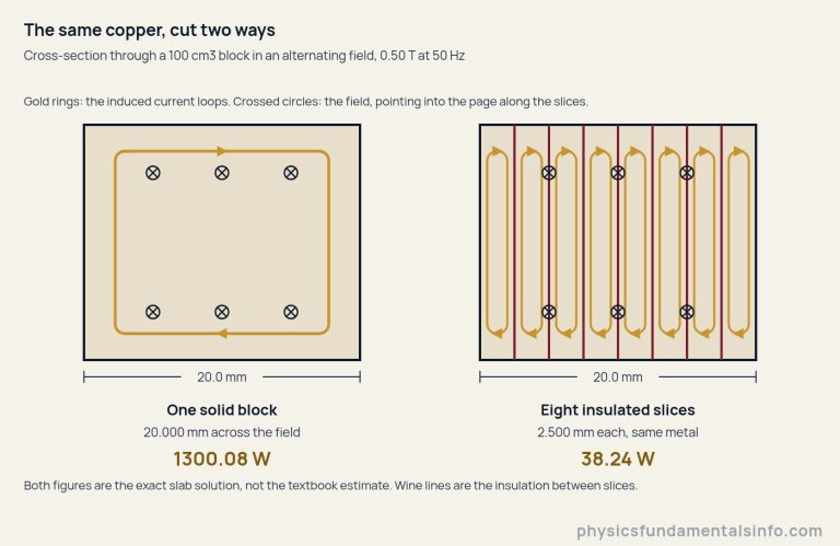
Now the result this page exists for. Cutting the block into forty insulated slices takes it from 1300.08 W to 1.53 W. The squared rule says forty slices should divide the loss by 40², which is 1600. What the metal actually delivers is a reduction of 849.79 times.
The shortfall is not a failure of lamination. Divide the two predictions, 1600 / 849.79 = 1.8828, and compare that with the amount by which the textbook formula overstated the solid block in the first place: 2447.82 / 1300.08 = 1.8828. The same number, to every figure printed.
That is the whole explanation, and it is worth stating plainly: the squared rule was not wrong about the slicing. It was wrong about the block you started from. Why it was wrong about that block is the next section.
Where the Eddy Current Formula Stops Being True
The derivation quietly assumed the field is the same everywhere across the thickness, and the eddy currents themselves make that false: their own field opposes the applied one, so the interior of a thick piece of metal is screened.
The length that decides whether you can ignore that is the skin depth.
Here μ0 is the permeability of free space, taken throughout this cluster as 4π × 10−7 N/A². NIST publishes a measured vacuum magnetic permeability that sits a hair away from that, far too close to move anything here: copper’s skin depth at 50 Hz comes out as 9.2255 mm on either figure.
In copper the skin depth falls as the frequency rises, as the square root demands: 20.6288 mm at 10 Hz, 9.2255 mm at 50 Hz, 6.5234 mm at 100 Hz, 3.2617 mm at 400 Hz and 2.0629 mm at 1000 Hz. Resistivity pulls the other way, which is why a poorer conductor is screened less.
Nichrome makes that concrete. The same solid 20.0 mm block at 0.50 T and 50 Hz loses 1300.08 W in copper and only 37.38 W in nichrome — about 35 times less in the more resistive metal. Its skin depth is 74.650 mm, which dwarfs the block, so for nichrome the textbook formula is exact. Our guide to electrical resistance and resistivity covers where those material figures come from.
Solve the slab exactly, with no thin-sheet assumption at all, and a second closed form drops out. Write s for the thickness measured in skin depths, s = d/δ, and μ for the permeability of the metal, which equals μ0 here because the metal is non-magnetic.
Compare the two and you get a boundary rather than a warning. The textbook formula first reads 0.5 per cent high at 0.5929 skin depths, 1 per cent high at 0.7051, 5 per cent at 1.0545, 10 per cent at 1.2542 and 50 per cent at 1.8782. Those were scanned in steps of 0.0001 skin depths, not estimated.
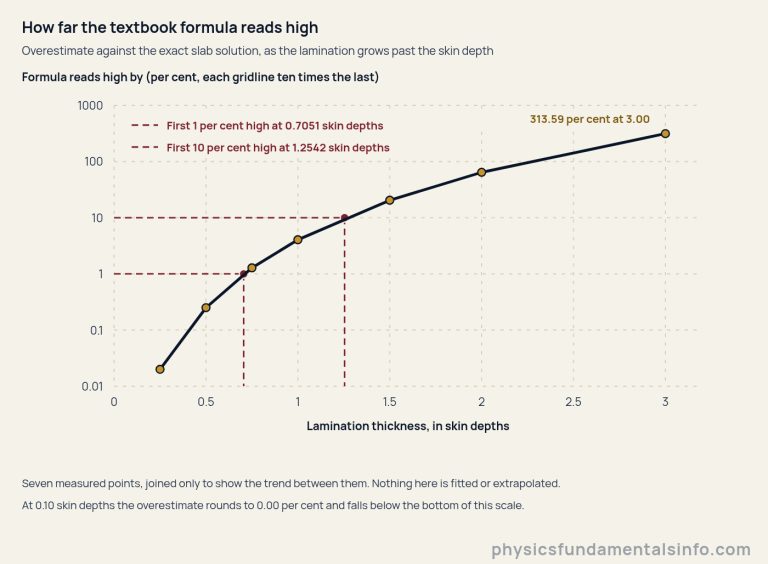
Here is the practical version of that chart. A real lamination sits far inside the 1 per cent line — the 0.500 mm copper sheet in the table above is only 0.0542 skin depths thick. A solid block usually does not.
How badly does it fail? At 400 Hz that same 20.0 mm copper block is 6.132 skin depths thick, and the textbook formula claims 156.7 kW where the metal delivers 4.062 kW — out by a factor of 38.56. Wind the frequency up to 1000 Hz and make the metal more conductive still and the gap widens to a factor of 330.7, which is the worst state the simulator above can be driven to.
Why a Thicker Block Can Lose Less Than a Thinner One
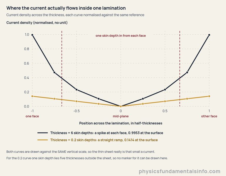
Past about 2.25 skin depths, making a piece of metal thicker lowers its loss per unit volume, because the extra metal sits in the screened interior and carries almost no current.
The peak sits at 2.2542 skin depths, found by scanning 200,000 thicknesses. By ten skin depths the loss per unit volume has fallen to 23.97 per cent of that peak. The textbook formula does the opposite and grows as d² for ever, which is precisely how the gap in the last section opened out to a factor of 330.7.
The clean way to see it is the total loss per unit of surface area, which saturates. For copper at 1 T and 50 Hz it reads 1.16354 × 10⁶ W/m² at five skin depths, 1.15333 × 10⁶ at ten, and 1.15319 × 10⁶ at both twenty and fifty. Past a few skin depths, adding metal adds volume and no extra loss whatsoever.
Once a sheet is that thick, the familiar scaling rules quietly stop applying. At two skin depths in copper, doubling the frequency multiplies the exact loss by 1.8762 rather than by 4. Doubling the thickness multiplies it by 0.6478 — the loss goes down. Doubling the resistivity multiplies it by 0.7067 instead of halving it.
None of that contradicts the formula. It just means the formula was never describing that sheet, and the only honest way to quote it is with a thickness in skin depths beside it.
Real-World Examples of Eddy Currents
Eddy currents show up wherever metal meets a changing field. Sometimes an engineer is working hard to suppress them; just as often, somebody is paying good money to produce them on purpose.
Transformer and motor cores, where the loss is pure waste
This is the calculation that fixes a lamination thickness. Thinner sheets mean less waste heat and a higher price, more insulation and less metal per centimetre of stack, so the choice is an economic one made against exactly the numbers in the table above.
Core loss is also a continuous draw whenever equipment is energised, doing useful work or not. One warning before those watts turn into money. The core loss a manufacturer quotes is two mechanisms added together: the eddy-current share this page computes, and hysteresis, the price of reversing the magnetisation of a ferromagnetic core twice in every cycle.
Hysteresis grows roughly with the first power of the frequency where the eddy-current loss grows with its square, so a quoted core-loss figure contains both and will not balance against anything computed here. Nothing on this page models it. Our guide to working out the cost of electricity turns a standing loss in watts into a bill.
Induction hobs and induction heating, where the loss is the point
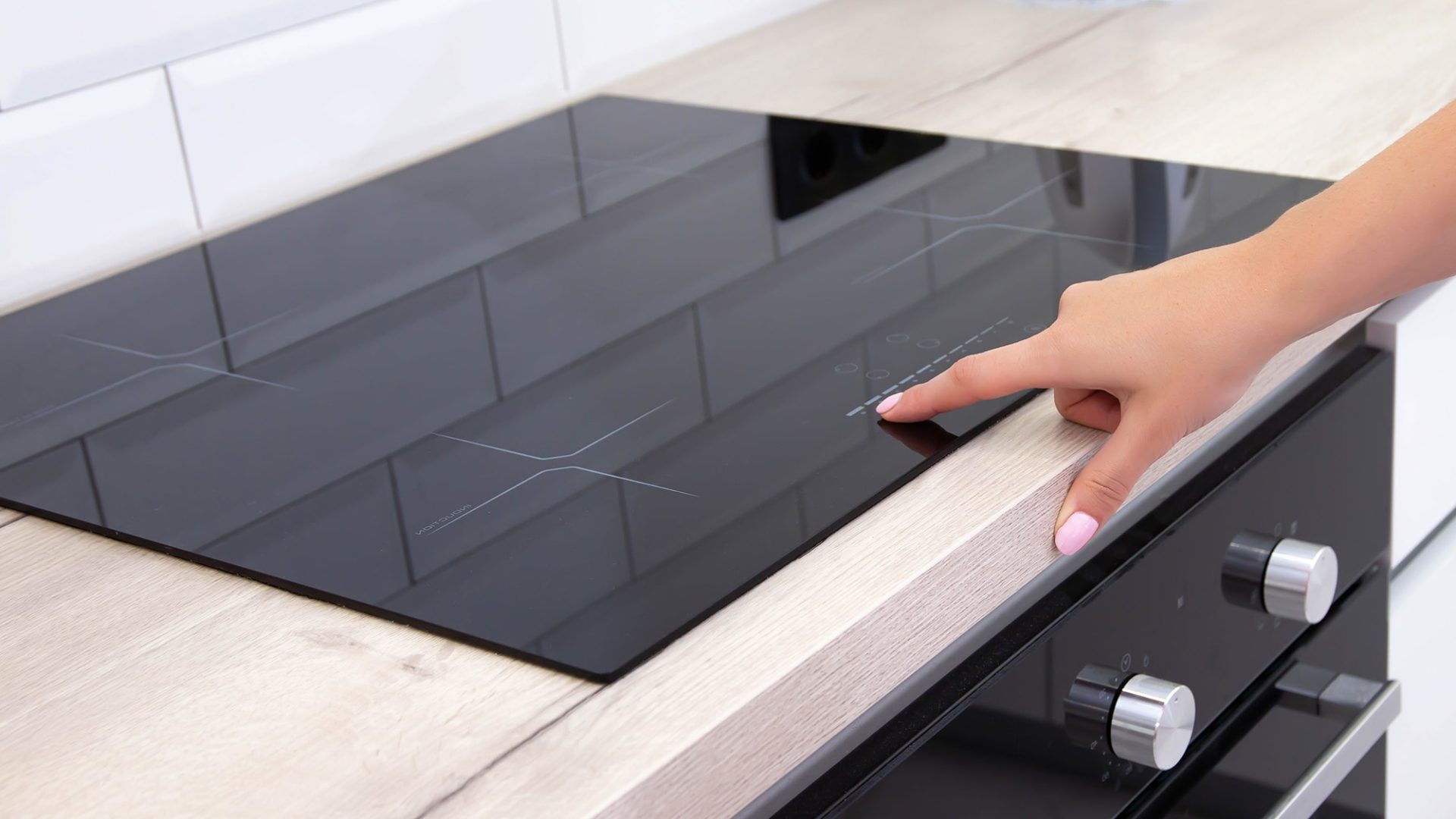
Flip the sign of the design goal and everything reverses. A coil under the glass drives a field into the pan, the eddy currents in the pan base do the cooking, and the hob stays comparatively cool because glass conducts nothing. Instead of thin sheets you want a thick, reasonably resistive base, and the frequency is chosen to put the skin depth where the heat is wanted.
Eddy-current brakes and damping
Drag a conductor past a magnet and Lenz’s law guarantees a retarding force with nothing in contact and nothing to wear out. Trains and roller coasters use it at scale; the spinning aluminium disc in an old electricity meter and the settling needle of a moving-coil instrument use it in miniature.
It is also why the magnet crawls down that copper pipe. This page deliberately puts no speed on that demonstration — the closed form for it rests on a dipole model and a numerical coefficient that this cluster could not derive from first principles, and an invented figure would be worse than none.
Metal detectors and non-destructive testing
A coil carrying alternating current induces eddy currents in any conductor nearby, and those currents push a field back into the coil and change what it measures. Do that crudely and you have a metal detector. Do it at a fixed, well-chosen frequency and you have eddy-current testing, which finds cracks and corrosion in aircraft skins and heat-exchanger tubes without touching them. What is read there is the change in the loss, which is why the skin depth matters so much.
Common Misconceptions About Eddy Currents
“Eddy currents are always a waste”
They are a waste in a transformer and the entire product in an induction furnace. Every application listed above except the first is somebody arranging for the loops on purpose — heating a pan, stopping a train, finding a crack in an aircraft skin. Treating the topic as pure loss is reading half of it.
“Forty slices must cut the loss 1600 times”
Forty slices cut it 849.79 times in the copper block measured here, not 1600. The squared rule is a fine description of thin sheets; the number it is being compared against, the loss in the solid block, is the one it gets wrong — by 88.28 per cent, because that block screens its own interior.
“Doubling the frequency always quadruples the loss”
It does while the sheet stays thin, and problem 6 below is exactly that case: a 0.500 mm copper sheet really does lose 64 times as much at 400 Hz as at 50 Hz. At two skin depths it does not, and the exact loss rises by 1.8762 instead of 4. A rule with a validity boundary is only useful if you carry the boundary around with it.
“A thicker piece of metal always burns more”
More in total, up to a point; more per unit volume, only up to 2.2542 skin depths. Beyond that the extra metal is screened, contributes almost no current, and the loss per cubic metre falls — which is the single most counter-intuitive thing in this whole topic.