An eddy current is a loop of current that a changing magnetic field drives inside a solid conductor, with no wire to guide it. This free eddy current loss calculator returns the power those loops waste in a thin lamination, P/V = π2B2f2d2 / (6ρ), and rearranges the same relation for the field, the frequency, the thickness or the resistivity. Beside the answer it prints the skin depth, the thickness in skin depths and the exact slab solution, so you can see at once whether the headline formula still applies.
Load a real case
Every button sets each unit menu it names — including the one the answer itself comes back in — moves the Solve for menu to whichever quantity its own case leaves unknown, and types the remaining figures. The line underneath quotes back whatever the widget works out from that, so nothing in it is stored text. Run the last four in order for a closed round trip: the loss that comes out of A more resistive metal goes back in and returns the thickness, the frequency, the field and the resistivity it started from.
Pick a case above, or type your own numbers.
What Is the Eddy Current Loss Calculator?
The eddy current loss calculator is a free online tool for the power an alternating magnetic field wastes inside a sheet of metal. Type the peak flux density, the frequency, the lamination thickness, the resistivity and a volume and it returns P/V = π2B2f2d2 / (6ρ), the classical thin-sheet loss per cubic metre, together with the total loss in that volume, the skin depth, the thickness measured in skin depths and the exact slab solution for comparison. Point the Solve for menu at the field, the frequency, the thickness or the resistivity instead and it rearranges the same relation, returning the positive root of the three arrangements that have two.
The headline relation is an approximation, and this page prints its boundary rather than hiding it: measured against the exact slab solution it is 1 per cent high once the sheet reaches 0.7051 skin depths, 5 per cent high at 1.0545 and 10 per cent high at 1.2542. A Textbook formula check chip says in words which side of those lines a given state falls on. The metal is assumed non-magnetic, with a relative permeability of one, so hysteresis loss is not modelled and no figure is offered for electrical steel.
| Symbol | Quantity | Default unit | Also accepts | Example value |
|---|---|---|---|---|
| P/V | Power loss per unit volume | W/m³ | kW/m³, MW/m³, W/cm³ | 15298.86595 |
| B | Peak flux density | T | mT, G | 0.50 |
| f | Frequency | Hz | kHz | 50 |
| d | Lamination thickness | mm | m, um, in | 0.500 |
| ρ | Resistivity | uOhm.cm | Ohm.m, uOhm.m, nOhm.m | 1.68 |
| V | Volume of metal | cm³ | m³, L | 100 |
How to use the eddy current loss calculator
- Choose the unknown. The Solve for menu opens on Power loss per unit volume. The other four choices are Peak flux density, Frequency, Lamination thickness and Resistivity, and whichever you pick vanishes from the boxes below.
- Type the peak flux density. Peak flux density takes T, mT or G and wants the peak of the alternating field rather than a root-mean-square value. It enters the relation squared, so −0.50 T returns exactly the same loss as 0.50 T; only a field of exactly zero is declined.
- Type the frequency. Frequency takes Hz or kHz and must be above zero. It does two jobs at once: it raises the loss as its square, and it shrinks the skin depth as one over its square root, which is why a thickness that is safe at 50 Hz may not be at 400 Hz.
- Type the lamination thickness. Lamination thickness takes mm, m, um or in, and it is the thickness of one sheet across the field, not the height of the stack. Forty half-millimetre sheets are 0.500 mm here, not 20.0 mm, and getting that wrong is the single commonest mistake on this page.
- Type the resistivity. Resistivity takes uOhm.cm, Ohm.m, uOhm.m or nOhm.m and opens on copper at 1.68 uOhm.cm. It must be above zero, because a perfect conductor would divide the formula by zero and a negative resistivity would hand back a negative power.
- Type the volume of metal. Volume of metal takes cm3, m3 or L, and it never moves the headline. It is there to turn a power density into watts in the Total loss in that volume chip, and it is the one field that can never be the unknown.
- Read the answer and the chips. The headline carries six significant figures while it stays a plain decimal, and turns into a four-figure exponential once it passes ten million in the unit the box is set to — the solid-block case reads
2.448e+7W/m3 until you switch the box toMW/m3, where it reads24.4782. The chips give the total loss, the skin depth, the thickness in skin depths, the exact slab loss, the ratio between the two, a worded validity check, and the loss at half the thickness and at twice the frequency. - Read the validity chip before you quote anything. Textbook formula check compares the headline with the exact slab solution and says in words when the headline is reading high. On the opening case the chip prints
reads 0.00 percent high - inside the 1 percent line at d over skin depth 0.7051; on the same copper in one 20.0 mm block it printsREADS HIGH by 88.28 percent - past the 10 percent line at d over skin depth 1.2542; read the exact slab figure instead. - Open Show working. The steps restate the relation, list your figures in the units the arithmetic really uses, print the top and the bottom of the fraction separately and divide them. The three modes that take a square root state plainly that a negative root exists and that the positive one is returned.
Four calculators here already own the neighbouring questions, and none of them can answer this one. The Faraday’s law calculator gives the EMF a changing flux drives round a coil of known turns, but it has no thickness and no resistivity; the resistivity calculator is R = ρL/A, the geometry of a wire, and it is where the 1.68 uOhm.cm copper figure on this page comes from. The magnetic field calculator and the magnetic force calculator both describe a steady field, and nothing is induced by a field that does not change.
The six-line derivation, the drawn loops and eight worked problems are all next door in the guide to eddy currents, which this tool is the arithmetic half of. If the direction of the induced loops is the unfamiliar part rather than their size, the guide to Lenz’s law is the place to start, and the Lenz’s law simulator shows the same opposition happening in a coil.
Two mistakes account for most wrong answers here. The first is typing the thickness of the whole stack instead of one sheet, which multiplies the answer by the square of the number of laminations; the second is quoting the headline without reading the validity chip, which is how a solid block gets reported as losing 88.28 per cent more than it really does.
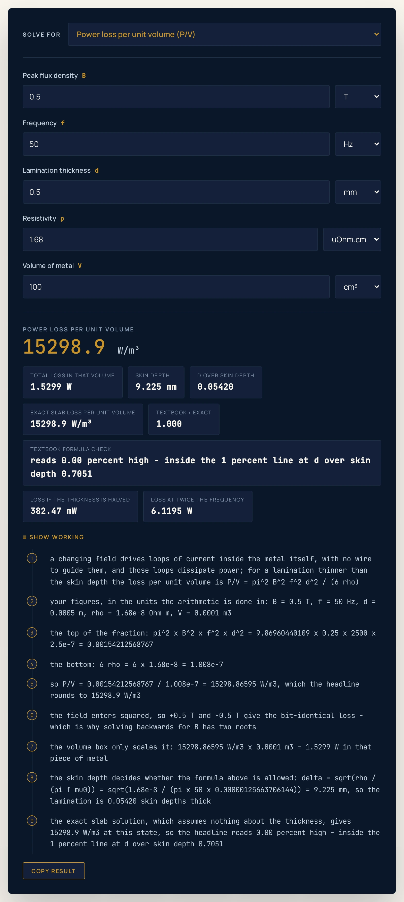
Exact slab loss per unit volume chip agree to every printed figure because the sheet is only 0.05420 skin depths thick — which is exactly the condition the formula was derived under.Worked example: change one thing at a time
The table starts at the defaults and moves one thing at a time: the thickness, then the frequency, then the metal, then which quantity is the unknown, then the unit the figures are typed in, and finally the entries the calculator declines. Rows 8 to 11 are the closed round trip, so the loss that leaves row 5 comes back in and returns the thickness, the frequency, the field and the resistivity it started from. Every Result, Total loss and Textbook / exact cell was read out of the running widget rather than worked out by hand, so where a cell and the tool ever part company, believe the tool.
| Step | Solving for | What you type | Result | Total loss | Textbook / exact |
|---|---|---|---|---|---|
| The page as it opens | Power loss per unit volume | 0.50 T, 50 Hz, 0.500 mm, 1.68 uOhm.cm | 15298.9 W/m³ | 1.5299 W | 1.000 |
| The same metal in one solid block | Power loss per unit volume | 0.50 T, 50 Hz, 20.0 mm, 1.68 uOhm.cm; answer box in MW/m³ | 24.4782 MW/m³ | 2.4478 kW | 1.883 |
| Aircraft frequency, 400 Hz | Power loss per unit volume | 0.50 T, 400 Hz, 0.500 mm, 1.68 uOhm.cm | 979127 W/m³ | 97.913 W | 1.000 |
| Four hundred hertz in the solid block | Power loss per unit volume | 0.50 T, 400 Hz, 20.0 mm, 1.68 uOhm.cm; answer box in MW/m³ | 1566.6 MW/m³ | 156.66 kW | 38.56 |
| A more resistive metal | Power loss per unit volume | 1.00 T, 50 Hz, 0.500 mm, 50.0 uOhm.cm | 2056.17 W/m³ | 205.62 mW | 1.000 |
| Halve the thickness | Power loss per unit volume | 1.00 T, 50 Hz, 0.250 mm, 50.0 uOhm.cm | 514.042 W/m³ | 51.404 mW | 1.000 |
| Nichrome, solid | Power loss per unit volume | 0.50 T, 50 Hz, 20.0 mm, 110 uOhm.cm | 373849 W/m³ | 37.385 W | 1.000 |
| How thin must it be? | Lamination thickness | 10000 W/m³, 1.00 T, 50 Hz, 50.0 uOhm.cm | 1.10266 mm | 1.0000 W | 1.000 |
| How fast was it driven? | Frequency | 2056.167584 W/m³, 1.00 T, 0.500 mm, 50.0 uOhm.cm | 50 Hz | 205.62 mW | 1.000 |
| How strong was the field? | Peak flux density | 2056.167584 W/m³, 50 Hz, 0.500 mm, 50.0 uOhm.cm | 1 T | 205.62 mW | 1.000 |
| What metal was it? | Resistivity | 2056.167584 W/m³, 1.00 T, 50 Hz, 0.500 mm | 50 uOhm.cm | 205.62 mW | 1.000 |
| The field typed in millitesla | Power loss per unit volume | 500 mT, 50 Hz, 0.500 mm, 1.68 uOhm.cm | 15298.9 W/m³ | 1.5299 W | 1.000 |
| The thickness typed in microns | Power loss per unit volume | 0.50 T, 50 Hz, 500 um, 1.68 uOhm.cm | 15298.9 W/m³ | 1.5299 W | 1.000 |
| A negative field, same loss | Power loss per unit volume | -0.50 T, 50 Hz, 0.500 mm, 1.68 uOhm.cm | 15298.9 W/m³ | 1.5299 W | 1.000 |
| Zero frequency is declined | Power loss per unit volume | 0.50 T, 0 Hz, 0.500 mm, 1.68 uOhm.cm | no answer | — | — |
| Zero field is declined | Power loss per unit volume | 0 T, 50 Hz, 0.500 mm, 1.68 uOhm.cm | no answer | — | — |
| A negative resistivity is declined | Power loss per unit volume | 0.50 T, 50 Hz, 0.500 mm, -1.68 uOhm.cm | no answer | — | — |
Rows 1 and 2 are the whole point of lamination, and they are the same 100 cm3 of copper in the same field. The headline reads 15298.9 W/m3 for the 0.500 mm sheet and 24.4782 MW/m3 for the one 20.0 mm block — but the block sits at 2.168 skin depths, where the last column shows the formula running 88.28 per cent high. Its exact slab chip reads 1.300e+7 W/m3 instead, and that, not the headline, is the figure to compare the sheet against.
Rows 3 and 4 raise the frequency to 400 Hz, eight times the mains figure, and the thin sheet duly loses 64 times as much because the relation squares the frequency. The block does not follow. Its skin depth falls from 9.225 mm to 3.262 mm, so the same 20.0 mm is now 6.132 skin depths and the headline overstates the loss by a factor of 38.56.
Rows 5 to 7 change the metal. Row 5 posits a 50.0 uOhm.cm metal, nearly thirty times the resistivity of copper, and the thin-sheet relation divides the loss by that same factor because it goes as one over rho — the relation restated, not a finding. Nichrome at 110 uOhm.cm keeps even a solid 20.0 mm block inside the 1 per cent line, and row 6 halves row 5’s thickness and quarters its loss for the same kind of reason.
Rows 8 to 11 read the relation backwards in each of the four remaining modes. Asking for a loss of 10000 W/m3 gives a maximum thickness of 1.10266 mm, and the last three take the 2056.167584 W/m3 that row 5 produces and return 50 Hz, 1 T and 50 uOhm.cm exactly. Three of those four rearrangements have a negative root as well, which the calculator discards.
Rows 12 to 14 are the unit menus and the sign. 500 mT is the same field as 0.50 T and 500 um is the same sheet as 0.500 mm, so both reproduce row 1 to the last digit. So does a field of −0.50 T, because the relation squares it.
Rows 15 to 17 sit on the edge of the domain and are refused there. A frequency of zero, a field of zero and a negative resistivity are all declined rather than answered, because the bare formula returns exactly 0 W/m3 for the first two and a negative power for the third, and a plausible-looking number is far more dangerous than a refusal.
Formula and symbol reference
The calculator uses one relation in five arrangements, and carries a second one beside it as a check. Apply Faraday’s law to a rectangular loop inside a slab of non-magnetic metal, average the dissipation across the thickness and over a cycle, and the loss per unit volume comes out as P/V = π2B2f2d2 / (6ρ). There is no fitted constant in that: the 6 is 12 times 2, the 12 from the second moment of the thickness and the 2 from the mean square of a cosine.
The second relation is the skin depth, δ = sqrt(ρ / (πfμ0)), and it is the yardstick rather than a decoration. The derivation above quietly assumed that the field is the same all the way through the sheet, which is true only while the thickness is small compared with δ. Solving the same slab exactly, with no such assumption, gives P/V = B2(sinh s − sin s) / (σμ2dδ(cosh s + cos s)) with s = d/δ, and that is the figure in the exact slab chip.
Each rearrangement below is the exact form one of the Solve for modes evaluates, which is why they are set out rather than left implied. Reading the relation backwards gives B = sqrt(6ρ(P/V) / (π2f2d2)), f = sqrt(6ρ(P/V) / (π2B2d2)) and d = sqrt(6ρ(P/V) / (π2B2f2)), each with a second, negative root that the calculator discards; solving for the resistivity is linear, ρ = π2B2f2d2 / (6(P/V)), and has one root only.
| Symbol | Meaning | SI unit | Values used on this page |
|---|---|---|---|
| P/V | Power lost per unit volume of metal. It is a power DENSITY, so it does not depend on how much metal there is; the Total loss chip multiplies it by the volume you entered | watt per cubic metre | Boxes take W/m3, kW/m3, MW/m3 or W/cm3: 15298.9 on the opening case, 24.4782 MW/m3 for the same metal in one block. |
| B | Peak flux density of the alternating field, taken along the lamination. It enters squared, so its sign is lost and the two signs give the identical loss | tesla, T | Boxes take T, mT or G: 0.50 on the opening case, 1.00 on the resistive-metal case, and 500 mT is the same field as 0.50 T. |
| f | Frequency of the alternating field. It also enters squared, and it sets the skin depth, so raising it both raises the loss and lowers the thickness at which the formula stops working | hertz, Hz | Boxes take Hz or kHz: 50 on the opening case, 400 on the aircraft case. |
| d | Thickness of ONE lamination, measured across the field. Not the height of the stack, and the quantity the whole topic turns on | metre; millimetres on this page | Boxes take mm, m, um or in: 0.500 on the opening case, 20.0 for the solid block, 500 um is the same sheet as 0.500 mm. |
| ρ | Resistivity of the metal. A more resistive metal carries a smaller eddy current for the same induced field, so the loss falls as one over rho | ohm metre; microhm-centimetres on this page | Boxes take uOhm.cm, Ohm.m, uOhm.m or nOhm.m: 1.68 is copper, 110 is nichrome, and 50.0 is a posited metal rather than a named one. |
| V | Volume of metal in the field. It never changes the headline and can never be the unknown; it turns the power density into watts | cubic metre; cubic centimetres on this page | Boxes take cm3, m3 or L: 100 cm3 on every row of the table above. |
| δ | Skin depth, the distance the alternating field reaches into the metal. The yardstick the thickness has to be measured against, and printed as a chip rather than typed | metre; millimetres on the chip | Computed, never typed: 9.225 mm for copper at 50 Hz, 3.262 mm at 400 Hz, 50.329 mm for a 50.0 uOhm.cm metal at 50 Hz. |
| μ0 | Permeability of free space, and the only constant this page types. The metal is assumed non-magnetic, so its own permeability is taken as this same value | henry per metre | A constant: 4π × 10−7 H/m. The SI 2019 value 1.25663706212e-6 gives the same 9.225 mm skin depth. |
The physics: why thin sheets win, and where the formula stops telling the truth
Put a lump of metal in an alternating field and Faraday’s law does not care that there is no wire. Every closed path inside the metal encloses a changing flux, so an EMF appears round every one of them, and the metal’s own conductivity turns that EMF into current. The guide to electromagnetic induction covers the EMF itself; what this page adds is what happens once that EMF has nothing but metal to drive current through.
The direction is settled by Lenz’s law: the loops flow the way that opposes the change that made them. That single sentence is the whole of the qualitative story and it belongs to the Lenz’s law article rather than to this page. What Lenz’s law cannot tell you is how much power the loops burn, because it contains neither a thickness nor a resistivity.
The size comes from the geometry. A loop a distance x from the mid-plane of the sheet encloses a flux proportional to x, so the induced electric field grows linearly outwards and the dissipation, which goes as the square of it, grows as x squared. Average that across the thickness and the answer picks up a factor of d2/12, which is where the square comes from.
That square is why lamination works so well, and why the benefit is easy to overstate. Slice a block into ten insulated sheets and each sheet is a tenth as thick, so each loses one hundredth as much per unit volume while the volume of metal is unchanged — a hundredfold cut in total. The insulating varnish does no physics of its own; it simply stops the loops from closing across the whole block.
Now the part that a page written from memory usually gets wrong. The derivation assumed that the field is the same everywhere across the thickness, and the eddy currents themselves make that false: their own field opposes the applied one, so beyond about a skin depth the interior of the metal is screened and carries almost nothing. The thin-sheet formula keeps growing as d2 for ever; the metal does not.
The boundaries were measured rather than guessed, and they are the most useful numbers on this page. The textbook formula is good to 0.5 per cent while the thickness stays under 0.5929 skin depths, to 1 per cent under 0.7051, to 5 per cent under 1.0545, and by 1.2542 it is 10 per cent high. Real laminations sit far inside all of that; a solid block usually does not.
Past those lines the disagreement stops being academic. The same 100 cm3 of copper in one 20.0 mm block sits at 2.168 skin depths, where the headline reads 88.28 per cent high, and at 400 Hz the same block sits at 6.132 skin depths and the headline is out by a factor of 38.56. The exact slab chip is unaffected by any of this, because it makes no thin-sheet assumption at all.
There is a genuine surprise hiding in that. Because only a skin of order δ carries any current, the loss per unit volume of a thick slab peaks at 2.2542 skin depths and then falls: by ten skin depths it is down to 23.97 per cent of its peak. Adding metal below the skin adds volume without adding loss, which is the exact opposite of what d2 promises.
It also means the familiar scaling rules quietly stop applying once a sheet is thick. Doubling the frequency at two skin depths multiplies the exact loss by 1.8762 rather than by 4; doubling the thickness there multiplies it by 0.6478, so the loss goes down; and doubling the resistivity multiplies it by 0.7067 rather than halving it. The two what-if chips on this page are the thin-sheet rule restated and carry none of that, which is why the validity chip sits between them and the headline.
Finally, a limit worth naming before it bites. Everything above is about a non-magnetic metal, and a real transformer core is not one — it is a ferromagnetic alloy whose relative permeability runs into the thousands, which shrinks its skin depth by the square root of that same factor. That is why real laminations are a fraction of a millimetre thick, and it is also why no figure on this page is offered for any steel.
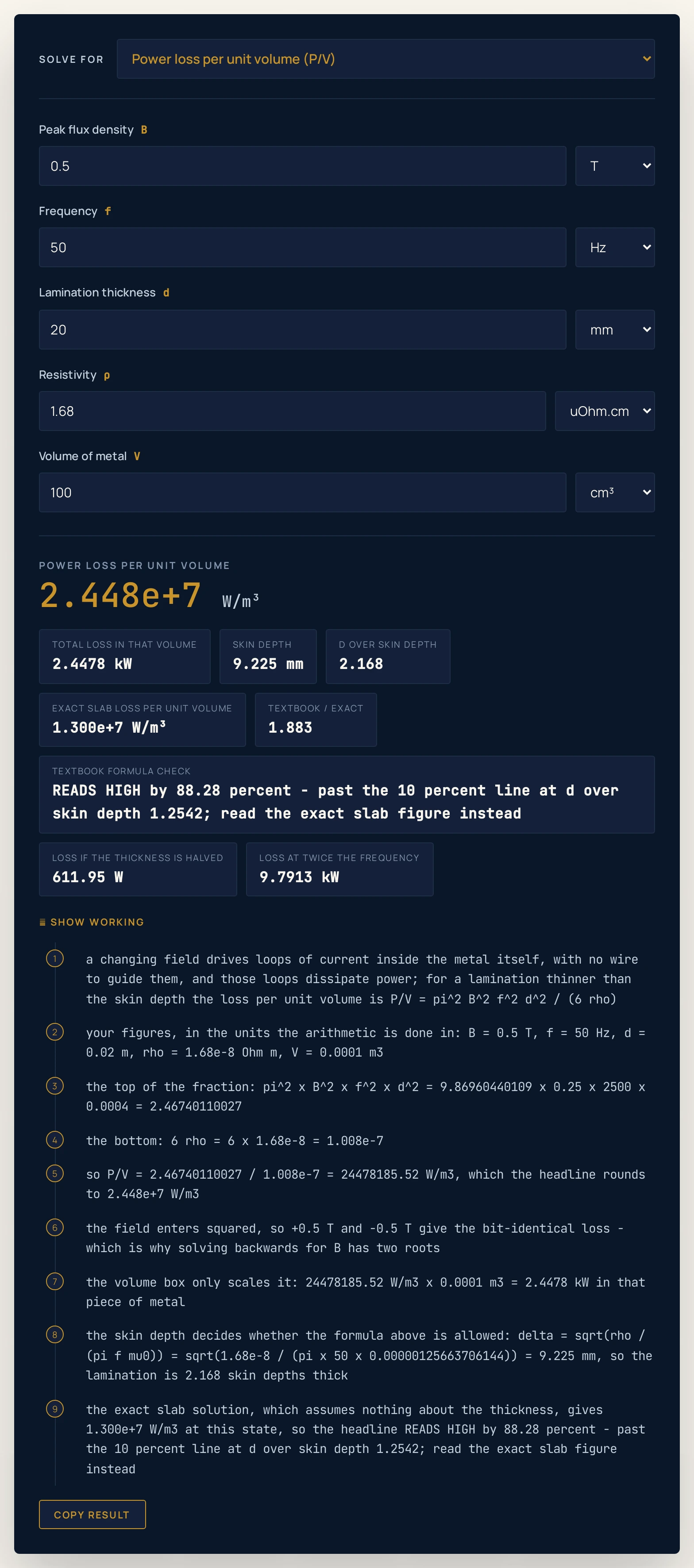
2.168 skin depths the chip reads READS HIGH by 88.28 percent against the exact slab solution — the one state on this page where the formula in the banner should not be quoted. This is also the four-figure exponential the headline falls back to above ten million: switch the answer box to MW/m3 and the same number reads 24.4782.Where the eddy current loss calculator breaks down
The arithmetic is exact to the last digit a double can hold. What fails is a thin-sheet formula being asked about a thick sheet, a ferromagnetic core being described by a non-magnetic model, or a stack thickness being typed where one lamination belongs.
- The headline formula is an approximation, and its boundary is printed for you
- Everything in the banner rests on the field reaching right through the sheet, which stops being true once the thickness approaches the skin depth. Measured against the exact slab solution, the formula is 1 per cent high at 0.7051 skin depths, 5 per cent high at 1.0545 and 10 per cent high at 1.2542, and it keeps going: at 2.168 skin depths it is 88.28 per cent high and at 6.132 it is out by a factor of 38.56. That is why the Textbook formula check chip exists and why it is worded rather than numeric.
- The metal is non-magnetic, with a relative permeability of one
- The skin depth used here is
sqrt(ρ / (πfμ0)), with no relative permeability in it. A ferromagnetic core has a relative permeability in the thousands, so its skin depth is smaller by the square root of that factor and a sheet that looks thin in millimetres may be several skin depths thick. This page gives no figure for electrical steel or any other magnetic alloy, because none was measured for it; treat any such number you find elsewhere as needing its own source. - Hysteresis is a separate loss and is not modelled at all
- A real ferromagnetic core loses energy twice over: once to eddy currents, which is what this page computes, and once to hysteresis, the work of turning the magnetisation round and back each cycle. Hysteresis rises roughly in proportion to the frequency while eddy-current loss rises as its square, so which one dominates depends on where you are. A core loss quoted by a manufacturer normally includes both, and comparing it with this page’s figure alone will not balance.
- The field is assumed uniform, sinusoidal and along the sheet
- One frequency, one amplitude, one direction, lying in the plane of the lamination. A square wave, a field with harmonics on it, a field that varies along the sheet or one with a component through the thickness all break the derivation, and a pulse-width-modulated drive is none of these things. The peak flux density box wants a peak rather than a root-mean-square figure, which for a sine wave differs by a factor of about 1.414 and therefore by a factor of two in the answer.
- The laminations are perfect, and real ones are not
- The model treats each sheet as perfectly insulated from its neighbours, infinitely wide and long compared with its thickness, and takes up no room for the insulation itself. A real stack has a stacking factor below one, burrs at the cut edges that can short neighbouring sheets together, and edges where the current has to turn round. All three push a real core above the figure here, and the edge effect matters most for a narrow sheet.
- Type one lamination, not the whole stack
- The thickness box is the thickness of a single sheet measured across the field. Typing the height of a forty-sheet stack instead of one sheet multiplies the answer by 1600, which is the square of the count, so it does not look like a slip — it looks like a catastrophe in the design. The volume box is where the size of the stack belongs, and it scales the total loss without touching the headline density.
- Three of the five modes have a second, negative root
- Solving for the field, the frequency or the thickness means taking a square root, and the relation squares all three, so the negative root satisfies it exactly as well as the positive one. The calculator returns the positive root and the working says so on its own line. Solving for the resistivity is linear and has a single root, and solving forwards for the loss has no ambiguity at all.
- Zero is refused wherever it would look like an answer
- At zero frequency, zero thickness or zero field the bare formula returns exactly 0 W/m3, which on screen is indistinguishable from a broken tool, so all three are declined as inputs. A resistivity of zero divides by zero and a negative one returns a negative power, so the guard there is strictly greater than zero rather than merely not equal to it. The refusal sits at zero and not near it: a hundredth of a hertz is a legal frequency and answers normally.
- Do not divide the two power figures on screen
- The headline and the exact slab chip are each rounded on their own before they are printed, and the ratio between two rounded numbers is not the rounded ratio. Over a grid of 60,000 states spanning the field from 0.05 to 2.00 T, the frequency from 10 to 1000 Hz, five thicknesses and three metals, dividing the two printed strings fails to reproduce the printed ratio in 5,178 of them, 8.63 per cent. Read the Textbook / exact chip instead, which is computed from the unrounded values.
- The same applies to the skin depth chip
- The skin depth is printed to three decimal places in millimetres, and recomputing the thickness in skin depths from that printed figure disagrees with the printed d over skin depth chip in 9,520 of the same 60,000 states, 15.87 per cent. A worked instance: at 20 Hz in copper the chip reads 14.587 mm, from which a 1.00 mm sheet works out at 0.06855 skin depths, while the chip beside it reads 0.06856. Both chips are right; neither is a check on the other.
- Rounded figures in, rounded figures out
- The headline is rounded while the arithmetic behind it is not, so feeding a printed answer back in as an input moves the result slightly. The reverse presets here land exactly because they type the ten-figure value that Show working prints, not the rounded headline. That is also why the working prints every operand unrounded: each line can then be checked exactly as it stands.
- The two what-if chips are the formula restated, not a result
- Loss if the thickness is halved is a quarter of the total and Loss at twice the frequency is four times it, because the relation says
d2andf2. They are on the page because they are the two most useful things to know about a lamination, not because the tool discovered them, and they inherit the headline’s assumption: once a sheet is a skin depth or more thick, the real metal does not follow either rule. - The calculator measures nothing — you supply every figure
- Five numbers go in, one relation is rearranged, and the answer describes that idealised sheet and nothing else. It is not a measurement of a transformer, a motor or an induction hob, and the preset names are shorthand for the figures beside them rather than claims about any apparatus. Verify anything you mean to rely on against your own data before you quote it.
Where eddy-current loss is actually used
- Why transformer and motor cores are stacks of thin sheets
- This is the calculation that decides a lamination thickness. The loss goes as the square of the sheet, so halving it quarters the waste heat, and the only limits on going thinner are the cost of the sheet, the insulation between sheets and the fraction of the core volume it eats. Run the opening case, then run it again at 20.0 mm, and the difference between a stack and a lump is the whole of it.
- Why aircraft and high-frequency equipment laminate harder
- Aircraft electrical systems run at 400 Hz because a higher frequency lets a transformer do the same job with less iron, and switching supplies run far above that. The eddy-current loss rises as the square of the frequency, so the same sheet at 400 Hz loses 64 times as much as at 50 Hz, and the skin depth falls as well. Above a few kilohertz laminations give way to ferrites and to powdered-iron cores, whose resistivity is orders of magnitude higher.
- Induction hobs and induction heating, where the loss is the point
- Everything on this page is a description of waste until you want the heat, and then the same arithmetic runs in reverse: a coil drives a field into a pan and the eddy currents in the pan do the cooking. The design goal flips from thin sheets to a thick, reasonably resistive base, and the frequency is chosen to put the skin depth where the heat is wanted. Industrial induction hardening and metal melting are the same idea at much larger power.
- Eddy-current brakes and damping
- Drag a conductor through a field and the induced loops oppose the motion, which gives a braking force with no contact and nothing to wear out. It is used on trains and on roller-coasters, and in miniature on the aluminium disc of an old electricity meter and the needle of a moving-coil instrument. A magnet dropped down a copper pipe falls slowly for exactly this reason, and this page deliberately puts no number on that particular demonstration.
- Metal detectors and non-destructive testing
- A coil driven with alternating current induces eddy currents in any conductor nearby, and those currents push a field back into the coil and change what it sees. That is a metal detector; the same principle at a fixed, well-controlled frequency is eddy-current testing, which finds cracks and corrosion in aircraft skins and heat-exchanger tubes without touching them. What is being read there is the change in the loss, which is why the frequency and the skin depth matter so much.
- Counting the cost of the waste heat
- A core loss is a continuous draw whenever the equipment is energised, whether or not it is doing useful work, which is why transformer standby losses are regulated. Take the Total loss in that volume chip for the whole core volume and the electricity cost calculator will turn those watts into a yearly bill. The heat also has to be carried away, so the same figure sizes the cooling.
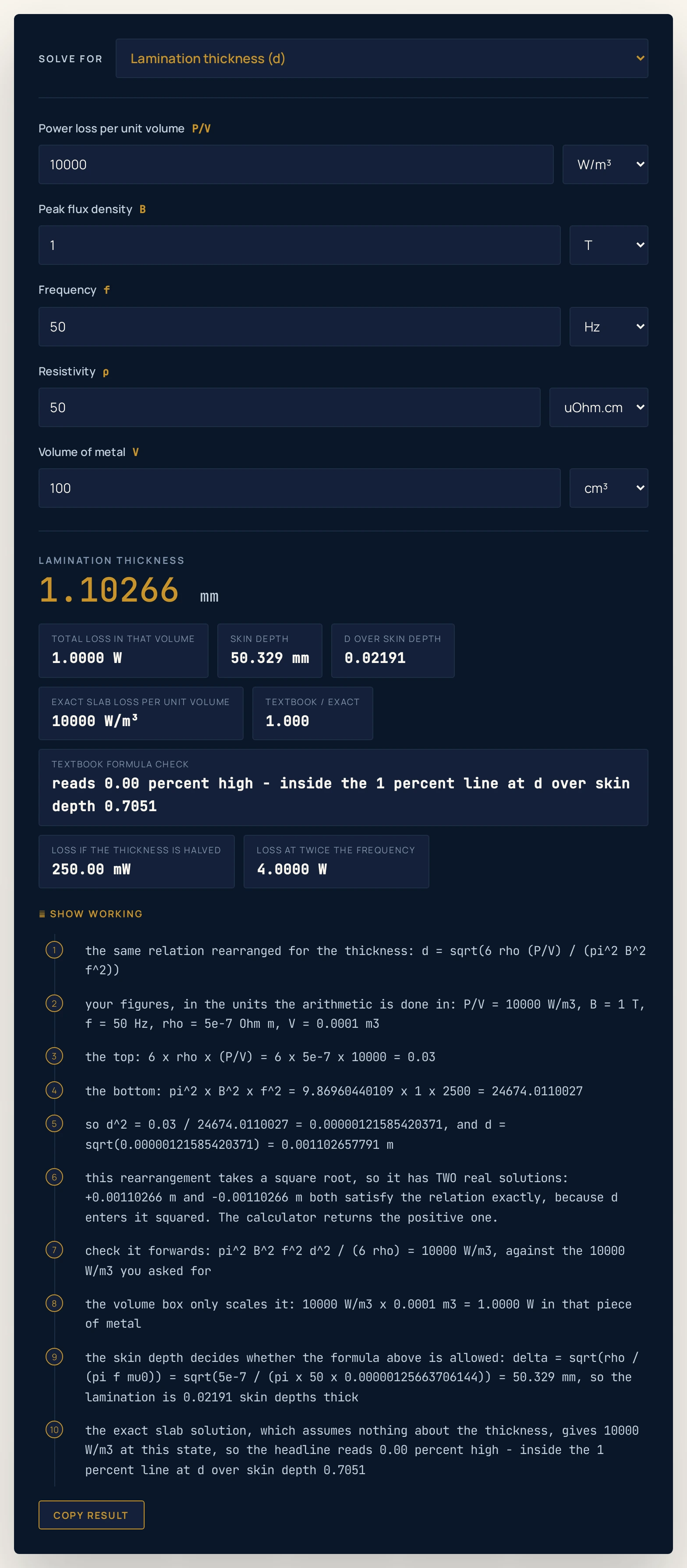
−0.00110266 m satisfies it just as exactly; the calculator returns the positive root and the working says so on its own line.Where to go next
For the derivation in full, with the loops drawn, the screening explained and eight worked problems, read why metal cores are cut into slices. For the law that fixes which way the loops turn, the guide to Lenz’s law is the companion piece, with the Lenz’s law simulator beside it.
Three more are worth a bookmark. The guide to electromagnetic induction sets out the EMF this page turns into watts; the Faraday’s law calculator handles that EMF in a coil of known turns; and the resistivity calculator is where the copper and nichrome figures used here come from. The whole physics lab library is open too, and the site search will find anything this page has not.
Frequently asked questions
What does the eddy current loss calculator work out?
It works out the power that an alternating magnetic field wastes as eddy currents inside a thin sheet of metal, from the formula P/V = pi squared times B squared times f squared times d squared, all divided by six times rho. Enter the peak flux density, the frequency, the lamination thickness, the resistivity and a volume, and it returns the loss per cubic metre along with the total loss in that volume, the skin depth, the thickness in skin depths and the exact slab solution for comparison. Point the Solve for menu at any of the five quantities instead and it rearranges the same relation, so a measured loss can give you back the field, the frequency, the thickness or the resistivity.
What is an eddy current?
An eddy current is a loop of electric current that a changing magnetic field drives inside a solid conductor, with no wire to guide it. Faraday induction says a changing flux produces an electromotive force around any closed path, and a lump of metal is full of closed paths, so the current simply circulates inside the metal. Lenz law fixes the direction: the loops always flow the way that opposes the change that made them.
Why does cutting a core into laminations help so much?
Because the loss goes as the square of the thickness of each sheet, not as the square of the whole block: cut a block into ten insulated sheets and each is a tenth as thick, so the thin-sheet formula says the total falls a hundredfold. Real metal gives less than that, and the reason is the block you started from rather than the sheets you cut it into: at 20.0 millimetres of copper at mains frequency the formula reads 88.28 per cent high, so it was overstating the loss before any cutting happened. Lamination still works, and it is why transformer and motor cores are stacks of thin sheets with varnish between them rather than solid lumps of metal.
Why is the answer sometimes much larger than the truth?
Because the headline formula assumes the field reaches right through the sheet, and past a certain thickness the eddy currents themselves screen it out of the middle. The measured boundaries are in the tool: the formula is good to one per cent while the thickness stays under about 0.7051 skin depths and to five per cent out to about 1.0545, and by 1.2542 it is already ten per cent high. The Textbook formula check chip says which side of those lines you are on, and the exact slab chip gives the unapproximated answer.
What is the skin depth and why is it printed here?
The skin depth is the distance an alternating field penetrates into a conductor before it has fallen to about 37 per cent of its surface value, and it is the square root of rho divided by pi times f times mu nought. It is printed beside every answer because it is the yardstick the thickness has to be measured against: what matters is not whether a sheet is thin in millimetres but whether it is thin in skin depths. Copper at mains frequency has a skin depth of 9.225 millimetres, so a half-millimetre lamination is comfortably inside it.
Why does solving for the field or the frequency have two answers?
Because the loss depends on the square of each of them, so a sign is lost on the way in and cannot be recovered on the way out. Plus 0.50 tesla and minus 0.50 tesla give a bit-identical loss, and the same is true of the frequency and the thickness, which means the rearranged equation has a positive and a negative real root. The calculator returns the positive root and the working says so; solving for the resistivity is linear and has only one root.
Does this include hysteresis loss?
No, and that is the biggest thing missing from any real core calculation done here. Hysteresis is a separate mechanism, the energy spent turning the magnetisation of a ferromagnetic material round and back each cycle, and it rises roughly in proportion to the frequency rather than to its square. This page models a non-magnetic metal with a relative permeability of one, so there is no magnetisation to turn and no hysteresis term at all.
Can I use it for a transformer core made of electrical steel?
Not directly, and the reason is worth understanding rather than working around. Electrical steel is ferromagnetic with a relative permeability in the thousands, which shrinks its skin depth dramatically and is exactly why real laminations are a fraction of a millimetre rather than centimetres thick. This page assumes a relative permeability of one, quotes no figure for any steel, and would need both the permeability and a hysteresis term before it could describe one.
Why do the two power figures on screen not divide to give the printed ratio?
Because each of them is rounded on its own before it is printed, and a ratio of two rounded numbers is not the rounded ratio. Over a grid of 60,000 states spanning the field, the frequency, the thickness and the resistivity, dividing the two printed power strings fails to reproduce the printed Textbook over exact figure in 5,178 of them, which is 8.63 per cent. Your arithmetic is fine in those cases; the display is rounded, so read the ratio chip rather than working it out from the two numbers above it.
References & formula source
- The relation P/V = pi^2 B^2 f^2 d^2 / (6 rho) follows in six lines from Faraday law applied to a slab of non-magnetic metal in a uniform alternating field lying along the sheet, with no fitted constant anywhere in it: the 12 in the denominator is the second moment of the thickness and the 2 is the mean square of a cosine.
- The exact slab result P/V = B^2 (sinh s - sin s) / (sigma mu^2 d delta (cosh s + cos s)), with s = d / delta, is the standard solution of the one-dimensional magnetic diffusion equation across the thickness, and it reduces to the relation above as s tends to zero. It is what the Exact slab chip prints.
- Bozorth, Ferromagnetism, and Stoll, The Analysis of Eddy Currents, for the classical lamination loss and for the screening that makes the thin-sheet formula fail once the thickness approaches the skin depth.
- Resistivities: 1.68e-8 Ohm m for copper and 1.1e-6 Ohm m for nichrome are the two figures already published on this site by the resistivity calculator. No other material is named with a value on this page, and in particular no figure is given for electrical steel, which is ferromagnetic and outside this model.
- mu0 = 4 pi x 1e-7 H/m is the constant typed into this calculator. The SI 2019 value 1.25663706212e-6 H/m is larger by 5.4438 parts in ten thousand million, and because the skin depth goes as one over the square root of the permeability, the length it produces moves by half of that, 2.722 parts in ten thousand million. Neither is visible at the precision printed here: both constants give a skin depth of 9.225 mm for copper at 50 Hz.
- Every figure quoted in the text above is a string this calculator printed for the inputs named beside it, a constant the page states, or a count measured over the 60,000-state grid described in the section on rounded figures.
- Further reading: Eddy current — Wikipedia