The dimensional analysis simulator is a free interactive lab with four sliders and eight readings, and three of those readings are kept deliberately apart. Three sliders set the trial exponents p, q and r; the fourth chooses which of eight derivations is on the bench. The three residual readings answer one base dimension each, so a wrong exponent shows up as M 0.25 on its own row rather than as a single refusal. On the pendulum the lab opens with they read M 0.00, L 0.00 and T 0.00 — already solved, and waiting to be broken.
Dimensional Analysis: Slide the Exponents Until the Dimensions Balance
A target quantity and three ingredients. A dimensional formula is a vector of three exponents over the base dimensions [M][L][T] — multiplying quantities adds those vectors, a power scales them — so demanding that a trial law Q = k X1p X2q X3r have the dimensions of the target is three linear equations in three unknowns, one per base dimension. Three sliders set p, q and r; the ledger draws each row's contributions against its target to a stated, fixed scale and highlights the residual, and the payoff curve plots the trial law against the exact physics over one decade with both normalised at the left edge, which removes the constant k and leaves only the slope. Homogeneous means necessary, not sufficient: one half of m v2 and twice m v2 have identical dimensions. The exponents this sim finds are exact; the constants are not its to give.
Load a real derivation in one click
Each button writes the four sliders and touches nothing else, which is exactly what your own hand would do. They are in the sim’s own order, because that order is three groups rather than a list, and each group is one claim you can watch instead of taking on trust.
Buttons one, two and three are the group the lab exists for: the same exponent triple 0.50, -0.50, 0.00 three times over, with The constant k reading 6.283, then 1.414, then 1.000. Buttons four to six are a solvable derivation each, where the first exponent comes out at 1.50, 1.00 and 1.00. Buttons seven and eight are the pair where the method declines to answer, in the two opposite ways it can.
Pick one of the eight derivations above, or drag the four sliders yourself.
What Is the Dimensional Analysis Simulator?
The dimensional analysis simulator is a free interactive physics lab that runs in your browser, with nothing to install and no sign-up. It treats a quantity’s dimensional formula as a vector of three exponents over mass, length and time, and gives you three sliders that set the exponents of a trial law. A fourth slider picks which of eight derivations you are working on.
The panel answers in four cards and four more compact readings. Trial dimensions is what your three exponents come to, Homogeneous? is yes or no, The law dimensions give prints the trial law itself, and The constant k gives the number the real physics carries. Beneath them sit the target and the three residuals, one per base dimension.
Those three residual readings are the reason this is a panel and not a verdict. They are kept apart rather than added up, because the three rows are independent constraints that can break one at a time: on the opening pendulum, push Exponent of mass m to 0.25 and the mass row reads M 0.25 while the other two stay byte-identical at L 0.00 and T 0.00. Move the gravity exponent to -0.25 instead and two rows break at once, L 0.25 and T -0.50.
So the residual tells you which ingredient is wrong, which a single pass-or-fail answer cannot. That is also what makes the lab usable as a workbench rather than a checker: you can walk one exponent in quarter steps and watch exactly one row respond.
The three exponent sliders are relabelled for each derivation, so they always name the real ingredient. On the opening case they read Exponent of length L, Exponent of gravity g and Exponent of mass m; on the third they read Exponent of tension F, Exponent of linear density mu and Exponent of length L. All three span -2.00 to 2.00 in steps of 0.25, which puts every exponent this subject needs on the grid exactly rather than near it.
Three of the eight derivations are the sharpest thing the lab has to show. A pendulum period, a fall time and the speed of a wave on a string all solve to the same exponent triple, 0.50, -0.50, 0.00 — and their constants read 6.283, 1.414 and 1.000. Identical exponents, answers a factor of 6.283 apart.
The fourth card is therefore the honest one. It never claims the constant came out of the exponents: its sub-line at the pendulum reads 2*pi for a small-amplitude pendulum - dimensions cannot produce it, and at the string it reads exactly 1 here, so dimensions happen to give the whole answer. The reach of the method is not uniform, and the panel says so case by case.
Card 2 carries the same discipline. It is labelled Homogeneous? and never correct, and its sub-line is every exponent matches the target - necessary, not sufficient at all eight derivations. One half of a mass times a speed squared and twice that same product have identical exponents, so the check passes both and the second one is four times too big.
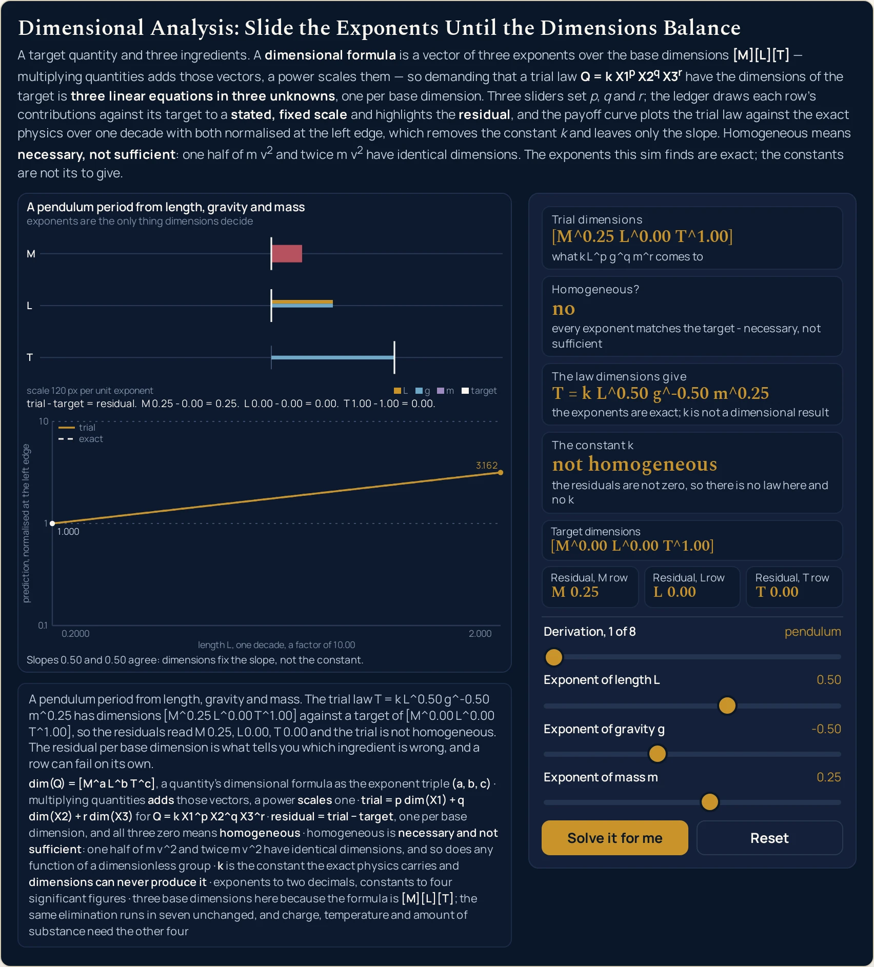
Two of the eight derivations exist to show the method refusing. On missing — a period from a length, a mass and an area — the time row reads T -1.00 for every triple you can reach, because the target needs a time and not one ingredient carries one. On ambiguous — a speed from a length, a gravity and a time — three different triples are all perfectly homogeneous, and the fourth card reads no single law rather than inventing one.
The drawing is a ledger above a graph, with no time axis anywhere in it. The ledger draws one row per base dimension: each ingredient’s contribution as a bar, the target beside it, and the residual marked. Its scale is chosen from a fixed ladder by the canvas width alone and never by the data, and the band underneath prints the rung in use, so the three rows stay comparable to each other at every width.
Below the ledger is the payoff. It plots what your trial law predicts against what the exact physics does, over one decade, with both normalised at the left edge — which removes the constant and leaves only the slope. Get the exponent right and the two curves lie on top of each other; move it a quarter step and they visibly separate.
Eight preset cases on the landing page write the four sliders for you, in three groups. The first three are the identical-triple group, the next three are a solvable derivation each, and the last two are the pair where the method refuses. Nothing in the lab needs starting: it opens on a pendulum that is already solved, so the button beside Reset opens offering to break it rather than to run anything.
Exponents print to two decimals and constants to four significant figures with the trailing zeros kept. Nothing beyond the exponent arithmetic is modelled: there is no Buckingham pi theorem and no counting of dimensionless groups, no dynamic similarity, no uncertainty propagation, no unit conversion and no natural or Planck units, and no figure is printed or implied for any of them.
| Control | Range | Step, default and what it moves |
|---|---|---|
| Derivation | one of eight | step 1; opens on the first, a pendulum period from length, gravity and mass. It chooses the target quantity and the three ingredients, so it rewrites the other three sliders with that case the moment it moves, and it relabels them to name the real ingredients. Its chip reads the case name and the position, from pendulum at Derivation, 1 of 8 to ambiguous at Derivation, 8 of 8 |
| First exponent | -2.00 to 2.00 | step 0.25; opens at 0.50. The trial exponent on whichever ingredient the derivation puts first, so its visible name changes from Exponent of length L to Exponent of tension F, Exponent of orbit radius r, Exponent of mass m or Exponent of density rho as you move along the eight cases. It drives the payoff curve on the six derivations whose leading ingredient is the first one |
| Second exponent | -2.00 to 2.00 | step 0.25; opens at -0.50. The trial exponent on the second ingredient, which is gravity on three of the eight cases and linear density, GM, speed or a mass on the rest. On the opening pendulum a quarter step on this one slider is the quickest way to break two residual rows at the same time, and on kinetic energy and dynamic pressure it is this slider, not the first, that the payoff curve is plotted against |
| Third exponent | -2.00 to 2.00 | step 0.25; opens at 0.00. The trial exponent on the third ingredient, which solves to exactly zero on six of the eight cases: that is the dimensional statement that the ingredient drops out. Moving it off zero on the pendulum breaks the mass row alone and leaves the length and time rows untouched |
| Solve or break | two labels | one button, and its label is not fixed. The lab opens on an already-solved triple, so the button reads Let me try and offers to move the exponents off the answer; once any slider is off the solved triple it reads Solve it for me and puts them back. Pressing it changes no target and no label |
| Reset | back to the opening setting | one button; it restores the derivation slider to the pendulum and the three exponents to 0.50, -0.50 and 0.00, which is the solved triple for that case |
How to use the dimensional analysis physics simulator
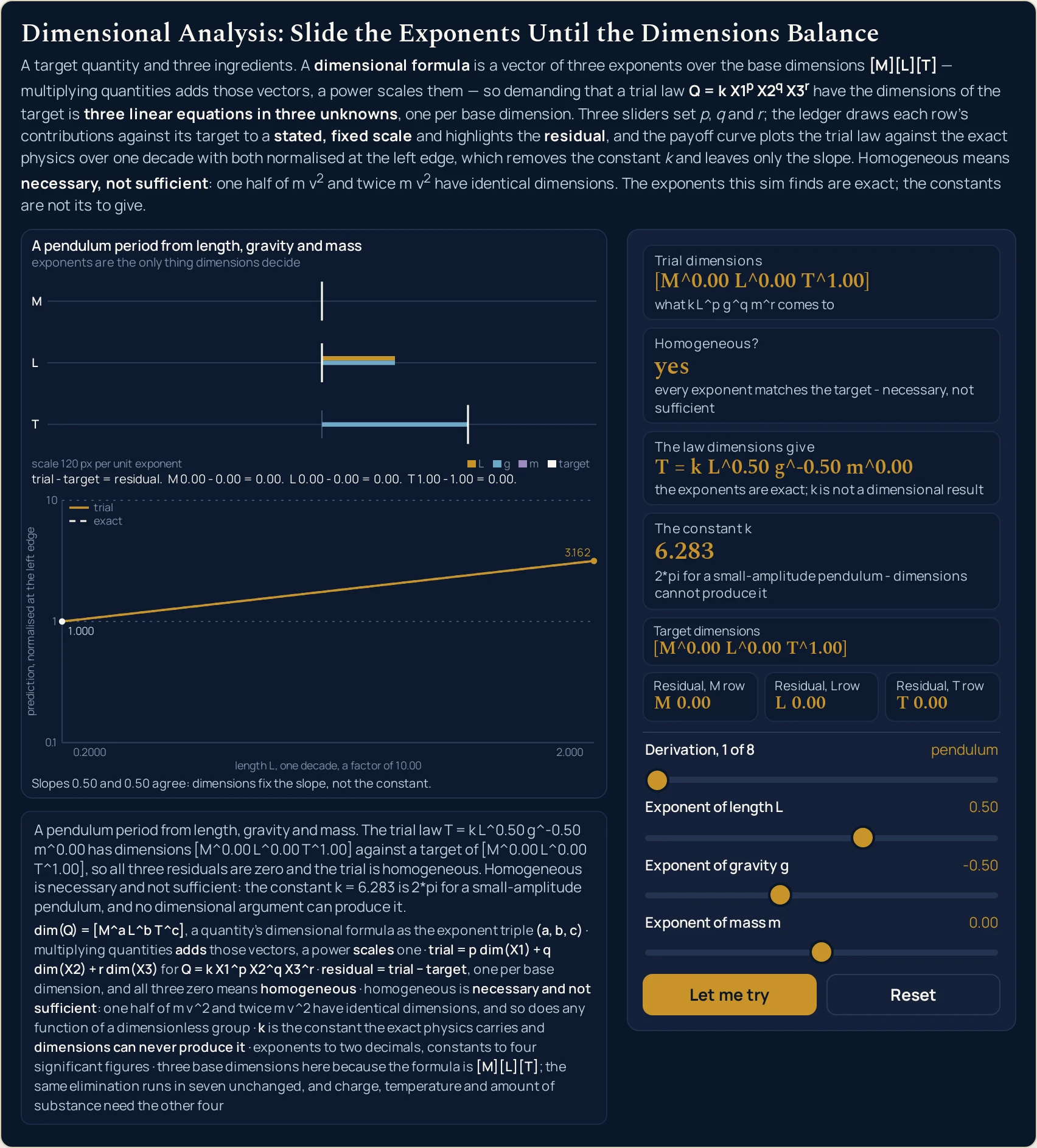
- Read the eight readings before you touch anything. The four cards are already answering for a pendulum period from length, gravity and mass: Trial dimensions [M^0.00 L^0.00 T^1.00], Homogeneous? yes, The law dimensions give T = k L^0.50 g^-0.50 m^0.00 and The constant k 6.283. The compact row beneath them reads [M^0.00 L^0.00 T^1.00], M 0.00, L 0.00 and T 0.00.
- Notice that the first card and the compact row’s first cell agree. Trial dimensions is what your three exponents come to; Target dimensions is what the chosen quantity actually is. Homogeneous means nothing more than those two strings matching, exponent for exponent, which is why the panel prints both rather than one verdict.
- Drag Exponent of mass m alone and watch one residual row move. At
0.25the three read M 0.25, L 0.00, T 0.00; at-0.25they read M -0.25, L 0.00, T 0.00. The length and time rows do not twitch, because the mass of a pendulum bob appears in no other equation of the three. - Now drag Exponent of gravity g instead and watch two rows go at once. One quarter step, to
-0.25, and the readings are M 0.00, L 0.25, T -0.50. Gravity carries both a length and a time, so a change in its exponent lands in two equations. That difference between the two sliders is the whole argument for three residual readouts. - Watch the button relabel itself while you do it. It reads Let me try when you arrive, because you arrive on a solved triple and the only useful offer is to break it. The moment any slider leaves that triple it reads Solve it for me, and pressing it writes the three exponents back. Nothing animates and there is nothing to start.
- Move Derivation, 1 of 8 one step and read the three slider labels. They change to name the new ingredients —
Exponent of height h, thenExponent of tension F, thenExponent of orbit radius r— and the three exponents are rewritten with that case’s own answer. A drag and a preset button therefore land on identical states. - Read the ledger in the upper half of the drawing, one row per base dimension. Each row draws the three ingredients’ contributions against the target and marks the residual. The scale is set by the width of the canvas and never by the numbers, and the band prints the rung in use — so a long bar is long because the exponent is big, not because the picture rescaled itself.
- Read the payoff curve underneath it, and move one exponent to break it. On the solved pendulum the trial and the exact curve lie on one another and the caption says they coincide. Take Exponent of length L from
0.50to1.00and they visibly separate, and the caption changes wording to say so. Both curves are normalised at the left edge, which removes the constant and leaves only the slope.
Dragging is the right way to find out which readings a control is allowed to move, and a poor way to hit an exact figure — all three exponent sliders step in quarters. Once you already have an exponent and want what it is worth, the dimensional scaling calculator takes typed input and solves the ratio in four directions; it has no ledger, no curve and no sliders, and this panel has no typed input and no inverse. The written guide to dimensional analysis in physics is where the subject itself is set out at length, with its worked problems.
Worked example: change one exponent at a time
Nothing in the three tables below was worked out here. Each row is a setting the lab was put into and then read back from, cell by cell, so every string in them is the panel’s own. The first table moves only the derivation slider, the second moves only one exponent at a time, and the third tries to break two cases that cannot be solved.
One: the eight derivations, each at its own answer
The derivation slider is the only control that moves between these rows. Each one carries its case’s solved triple, which is what the slider writes when you move it by hand.
| Derivation | Trial exponents | Trial dimensions | Homogeneous? | The law dimensions give | The constant |
|---|---|---|---|---|---|
| pendulum | 0.50, -0.50, 0.00 | [M^0.00 L^0.00 T^1.00] | yes | T = k L^0.50 g^-0.50 m^0.00 | 6.283 |
| freefall | 0.50, -0.50, 0.00 | [M^0.00 L^0.00 T^1.00] | yes | t = k h^0.50 g^-0.50 m^0.00 | 1.414 |
| string | 0.50, -0.50, 0.00 | [M^0.00 L^1.00 T^-1.00] | yes | v = k F^0.50 mu^-0.50 L^0.00 | 1.000 |
| orbit | 1.50, -0.50, 0.00 | [M^0.00 L^0.00 T^1.00] | yes | T = k r^1.50 GM^-0.50 m^0.00 | 6.283 |
| kinetic | 1.00, 2.00, 0.00 | [M^1.00 L^2.00 T^-2.00] | yes | E = k m^1.00 v^2.00 L^0.00 | 0.5000 |
| pressure | 1.00, 2.00, 0.00 | [M^1.00 L^-1.00 T^-2.00] | yes | q = k rho^1.00 v^2.00 L^0.00 | 0.5000 |
| missing | 0.00, 0.00, 0.00 | [M^0.00 L^0.00 T^0.00] | no | T = k L^0.00 m^0.00 A^0.00 | not homogeneous |
| ambiguous | 1.00, 0.00, -1.00 | [M^0.00 L^1.00 T^-1.00] | yes | v = k L^1.00 g^0.00 t^-1.00 | no single law |
Read the first three rows across and then down. Three unrelated problems — a swing, a drop and a plucked string — land on the identical trial exponents 0.50, -0.50, 0.00, and the last column reads 6.283, 1.414, 1.000. The exponents are the same to the last decimal and the constants span a factor of more than six. That single comparison is the clearest statement this panel makes about what dimensions do and do not give you.
The third row is the honest counterweight, and it is worth not skipping. For the wave on a string the constant is exactly 1.000, so there the exponents happen to be the entire answer. The method’s reach is not uniform, and the panel refuses to flatten that: the fourth card’s sub-line is different at every one of the eight cases. For the swing the sub-line names 2*pi for a small-amplitude pendulum, and the law with that constant in it belongs to the pendulum period formula guide rather than here.
Rows five and six are the same two exponents on quantities that are nothing alike. 1.00, 2.00, 0.00 gives [M^1.00 L^2.00 T^-2.00] for an energy and [M^1.00 L^-1.00 T^-2.00] for a pressure, with 0.5000 in front of each. That 0.5000 is exactly what the method cannot see: one half of a mass times a speed squared and twice that same product carry identical exponents, which is the point the mechanics formulas guide makes in words and this table measures. Row four stops at the exponent 1.50, and squaring that statement is the Kepler's laws guide, not this panel.
Two: one exponent at a time, with the derivation pinned on the pendulum
The derivation slider stays on Derivation, 1 of 8 in all nine rows, so Target dimensions is [M^0.00 L^0.00 T^1.00] throughout and never moves. Only the three residual columns are diagnostic.
| Trial exponents | Trial dimensions | Residual, mass row | Residual, length row | Residual, time row | Homogeneous? |
|---|---|---|---|---|---|
| 0.50, -0.50, 0.00 | [M^0.00 L^0.00 T^1.00] | M 0.00 | L 0.00 | T 0.00 | yes |
| 0.50, -0.50, 0.25 | [M^0.25 L^0.00 T^1.00] | M 0.25 | L 0.00 | T 0.00 | no |
| 0.50, -0.50, -0.25 | [M^-0.25 L^0.00 T^1.00] | M -0.25 | L 0.00 | T 0.00 | no |
| 0.25, -0.50, 0.00 | [M^0.00 L^-0.25 T^1.00] | M 0.00 | L -0.25 | T 0.00 | no |
| 1.00, -0.50, 0.00 | [M^0.00 L^0.50 T^1.00] | M 0.00 | L 0.50 | T 0.00 | no |
| 2.00, -0.50, 0.00 | [M^0.00 L^1.50 T^1.00] | M 0.00 | L 1.50 | T 0.00 | no |
| 0.50, -0.25, 0.00 | [M^0.00 L^0.25 T^0.50] | M 0.00 | L 0.25 | T -0.50 | no |
| 0.50, -0.75, 0.00 | [M^0.00 L^-0.25 T^1.50] | M 0.00 | L -0.25 | T 0.50 | no |
| 0.00, 0.00, 0.00 | [M^0.00 L^0.00 T^0.00] | M 0.00 | L 0.00 | T -1.00 | no |
Rows two and three move the mass exponent and nothing else responds. M 0.25 and M -0.25 while L 0.00 and T 0.00 stay byte-identical to row one. A mass appears in exactly one of the three equations, so an error in its exponent can only ever show up in one place, and the panel shows it in that one place.
Rows four to six move the length exponent, and again one row carries it all. L -0.25, L 0.50, L 1.50 while the mass and time rows hold at 0.00. Notice what the trial string does meanwhile: [M^0.00 L^1.50 T^1.00] at the bottom of that run, which is linear in the exponent you moved and in nothing else.
Rows seven and eight are the ones to read slowly. A quarter step on gravity breaks two rows at the same time — L 0.25 with T -0.50, then L -0.25 with T 0.50 — because gravity carries a length and a time together. Three rows that break in different combinations are three separate constraints, and that is why a single yes-or-no reading would throw away most of what the panel knows.
The last row sets every exponent to zero, and it is a useful place to stand. The trial collapses to [M^0.00 L^0.00 T^0.00], a pure number, and the only row left complaining is T -1.00: the target is a time and a pure number is not. Work back from that single residual and the quickest fix is to find an ingredient carrying a time, which is the habit the guide to solving physics problems places inside a wider routine.
Three: the two cases that cannot be solved, walked by hand
The seventh derivation asks for a period from a length, a mass and an area. The eighth asks for a speed from a length, a gravity and a time. Both fail, and they fail in opposite directions.
| Derivation | Trial exponents | Trial dimensions | Residual, time row | Homogeneous? | The constant |
|---|---|---|---|---|---|
| missing | 0.00, 0.00, 0.00 | [M^0.00 L^0.00 T^0.00] | T -1.00 | no | not homogeneous |
| missing | 0.50, 0.00, 0.00 | [M^0.00 L^0.50 T^0.00] | T -1.00 | no | not homogeneous |
| missing | 2.00, 0.00, -1.00 | [M^0.00 L^0.00 T^0.00] | T -1.00 | no | not homogeneous |
| missing | -2.00, 2.00, 1.00 | [M^2.00 L^0.00 T^0.00] | T -1.00 | no | not homogeneous |
| missing | -2.00, -2.00, -2.00 | [M^-2.00 L^-6.00 T^0.00] | T -1.00 | no | not homogeneous |
| ambiguous | 1.00, 0.00, -1.00 | [M^0.00 L^1.00 T^-1.00] | T 0.00 | yes | no single law |
| ambiguous | 0.50, 0.50, 0.00 | [M^0.00 L^1.00 T^-1.00] | T 0.00 | yes | no single law |
| ambiguous | 0.00, 1.00, 1.00 | [M^0.00 L^1.00 T^-1.00] | T 0.00 | yes | no single law |
The first five rows are five quite different triples and one unchanging column. T -1.00 at all of them, including both far corners of the grid. The target needs a time and not one of the three ingredients carries one, so the time row is unreachable rather than merely unfound — an exhaustive scan of tens of thousands of triples puts the best achievable residual at exactly 1, never 0.
That is a result the panel is reporting, not a fault in it. The reading has told you an ingredient is missing, and which one, because the row that will not close names the dimension you have left out. Swap the area for gravity — which is the first derivation — and the answer appears at once.
The last three rows are the opposite trouble, and the harder one to notice. Three triples that are nothing alike all read yes with every residual at zero: a speed as a length over a time, as the square root of a length times a gravity, and as a gravity times a time. All three are dimensionally perfect and they are different physical statements. The constant card prints no single law, which is the only honest thing left to print.
Formula and symbol reference
The lab prints its own definitions under the drawing, in plain ASCII, so that no radical sign and no subscript glyph is ever needed. Written out the same way: dim(Q) = [M^a L^b T^c] is a quantity’s dimensional formula as the exponent triple (a, b, c); multiplying quantities adds those vectors and a power scales one; the trial is p dim(X1) + q dim(X2) + r dim(X3); and the residual is trial - target, one per base dimension.
That is the entire model, and the square brackets are doing real work in it. [M] is the dimension mass, not the unit kilogram, and the two are not interchangeable: a dimension has no size, so there is nothing in this panel to convert. The units behind the brackets are set up in the guide to SI units in physics, which is a different question from the one this lab asks.
Nine rows follow and only four of them are something you drag. The rest are cards, cells of the compact row, or ideas the panel names without giving you a control for. For the sliders the last column gives the end stops and the step; for everything else it gives the strings the lab printed and the span it printed them over. A catalogue of nineteen named quantities with their exponent triples and coherent units is not repeated here — it sits in the dimensional formula table in the written guide, where prose can do something with it.
| Symbol or reading | Meaning | Unit | In this lab |
|---|---|---|---|
| dim(Q) | The dimensional formula of a quantity — the triple of exponents over mass, length and time that Trial dimensions and Target dimensions both print | a ratio of units, so dimensionless as written | the target string is set by the derivation slider alone and never moves when an exponent does: [M^0.00 L^0.00 T^1.00] on four of the eight cases, [M^1.00 L^2.00 T^-2.00] on kinetic energy, [M^1.00 L^-1.00 T^-2.00] on dynamic pressure. |
| a, b, c | The three exponents inside a dimensional formula — what the square brackets carry after the caret on M, L and T | pure numbers | printed to two decimals throughout, so a half-integer reads as exact: 0.50, -0.50, 1.50, 0.00. The most extreme trial string the tables above print is [M^-2.00 L^-6.00 T^0.00], at the bottom corner of the seventh derivation; drag all three exponents to the top of their range on the opening pendulum and the card reads [M^2.00 L^4.00 T^-4.00] at 2.00, 2.00, 2.00, which none of those tables reaches. |
| p | The trial exponent on the first ingredient — the second slider. It drives the payoff curve on six of the eight derivations, the six whose leading ingredient is the first one | a pure number | -2.00 to 2.00 in steps of 0.25, opening at 0.50. Its label is rewritten per derivation, from Exponent of length L to Exponent of tension F, Exponent of orbit radius r, Exponent of mass m and Exponent of density rho. |
| q | The trial exponent on the second ingredient — the third slider | a pure number | -2.00 to 2.00 in steps of 0.25, opening at -0.50. On the opening pendulum one quarter step on this slider alone is the quickest way to break two residual rows at once: L 0.25 and T -0.50. |
| r | The trial exponent on the third ingredient — the fourth slider, and the one that solves to zero on six of the eight cases | a pure number | -2.00 to 2.00 in steps of 0.25, opening at 0.00. Moving it off zero on the pendulum breaks the mass row alone: M 0.25 at 0.25, M -0.25 at -0.25, with L 0.00 and T 0.00 untouched. |
| residual | Trial exponent minus target exponent, one reading per base dimension — the three cells of the compact row after the target | pure numbers | all three read M 0.00, L 0.00, T 0.00 at any solved triple. The widest spread among the settings on this page is M -2.00, L -6.00, T -1.00, at the bottom corner of the seventh derivation. |
| k | The dimensionless constant the exact physics carries — the fourth card, The constant k. It is not a result of the exponents, and the card never pretends otherwise | dimensionless | 6.283, 1.414, 1.000, 6.283, 0.5000, 0.5000 on the six solvable cases, and the words not homogeneous and no single law on the other two rather than a number the trial has not earned. |
| the trial law | The law your three exponents amount to — the third card, The law dimensions give. It always carries the symbol k, at every setting |
depends on the target | the longest string the card prints is v = k F^0.50 mu^-0.50 L^0.00, on the third derivation. Its sub-line is byte-identical at all eight: the exponents are exact; k is not a dimensional result. |
| the derivation | Which of the eight problems is on the bench — the first slider. It sets the target, the three ingredients and the three slider labels at once | not a physical quantity | 0 to 7 in steps of 1, opening on the pendulum. The chip above it reads the case name and the position, Derivation, 1 of 8 through Derivation, 8 of 8. |
If you read one row twice, make it residual. It is the only reading on the panel that is three readings on purpose, and it is the one that turns a yes-or-no check into something you can debug.
The physics of dimensional homogeneity
The first claim the panel lets you test is that a dimensional formula is a vector and the algebra is addition. Nothing in the lab multiplies dimensions together: it scales each ingredient’s triple by its exponent and adds the three, one base dimension at a time. That is why Trial dimensions is exactly linear in the three sliders, and why doubling an exponent doubles exactly one contribution in each row.
The second claim is that homogeneity derives laws rather than only checking them. Three base dimensions give three equations; three dimensionally independent ingredients give exactly one exponent triple; and the derivation slider walks you through six cases where that happens. On the pendulum the mass exponent comes out as 0.00, which is the dimensional statement that a heavy bob and a light one of the same length keep the same period.
The third claim is the awkward one, and the panel is built around it rather than around the other two. Matching exponents is necessary and not sufficient, and the sub-line under the second card says so at all eight derivations. The lab offers three separate ways to watch it fail: an invisible constant on rows five and six of the first table, an unsolvable case, and a case with three right answers.
The fourth card is where that honesty is cashed out. It never claims the constant came out of the exponents — at the pendulum its sub-line reads 2*pi for a small-amplitude pendulum - dimensions cannot produce it, and at the string exactly 1 here, so dimensions happen to give the whole answer. Even that 2*pi is an approximation: the period depends on the amplitude, and an amplitude is a pure number, so no dimensional argument can see it at all.
Where this method breaks down
Every slider position this lab can reach is answered, and the arithmetic is not where it can let you down. The model behind it is, and so is the drawing. Nine limits sit under the readings on this page; three are choices the panel makes on purpose, and six are bounds on the method rather than on the panel.
- A dimensionless factor is completely invisible, and so is any function of one
- This is the limit everything else on the page hangs off. One half of a mass times a speed squared and twice that same product give byte-identical exponents, so the panel passes both and one of them is four times too big. The same blindness covers every pure number and every function of a pure number: an angle has no dimensions, so a period written as a constant times the square root of a length over a gravity times any function of the amplitude passes the check unchanged.
- The constants beside the exponents are quoted, not derived
- Five of the six solvable cases print a constant that is famous in its own right — 6.283, 1.414 and 0.5000 — and not one of them came out of this lab. They come from solving the real equation of motion or from measurement, and the fourth card’s sub-line names the source case by case. A reader who takes the exponent triple as “the formula” is wrong by whatever the constant happens to be, which across the first three rows of the first table is a factor of 6.283.
- Even the pendulum’s 2*pi holds only at small amplitude
- The constant the first derivation quotes is itself an approximation. The Wikipedia article on pendulum mechanics gives the small-angle condition as an amplitude much less than 1 radian, often cited as less than 0.1 radians or about 6 degrees, with an error of order the amplitude cubed. Measured from the series that source gives, the real period is 1.741 per cent above the small-angle value at 30 degrees and 0.04762 per cent above it at 5 degrees. Amplitude is dimensionless, so this panel cannot see any of that.
- Three dimensionally dependent ingredients leave the exponents unpinned
- Homogeneity gives one answer only when the three ingredients are dimensionally independent. On the eighth derivation they are not, and three different triples are all perfectly homogeneous, so the fourth card prints no single law. The underlying test is a determinant: it is exactly zero for both of the limits cases and non-zero for all six solvable ones. The panel does not print the determinant, and no reading on it should be treated as one.
- Three base dimensions are a choice, and four more exist
- This lab works in mass, length and time, which covers mechanics and stops there. The International System of Quantities has seven base quantities, and a dimension is written as a product of all seven with positive, negative or zero exponents. Charge, current, voltage and resistance need electric current; temperature and entropy need thermodynamic temperature; amount of substance needs its own. The same elimination runs in seven dimensions unchanged — there would simply be seven ledger rows instead of three.
- The Buckingham pi theorem is not here, and neither is similarity
- This panel solves one trial law with three ingredients and stops. Counting how many independent dimensionless groups a problem has, and what the rank of its dimensional matrix is, is a different and larger question that nothing in this lab answers and no reading on it estimates. Dynamic similarity and the groups it is built on belong to the guide to the Reynolds number, and no figure for any of it is printed or implied here.
- The ledger scale is set by the width of the canvas, and the band says which one
- The bars are drawn to a scale chosen from a fixed ladder by the canvas width alone, never by the numbers in them, so the three rows always stay comparable with each other. The band under the ledger prints the rung in use, and it is not the same rung on a phone as on a desktop. An auto-fitted scale would look tidier and would quietly make the comparison between rows meaningless, which is the one thing this drawing exists to support.
- A bar that runs off the window is clipped and marked, not shrunk
- The exponent sliders reach
-2.00and2.00, and a contribution at those ends can be longer than the row it lives in. When that happens the bar is cut at the edge and marked rather than redrawn to fit, because redrawing it would break the fixed scale that makes the rows comparable. Nothing is lost: the caption under the ledger and the compact row both still carry the exact figure. - The payoff curve answers for the leading ingredient only
- The lower scene plots the trial law against the exact physics over one decade of the leading ingredient only, with both normalised at the left edge. That is the first ingredient on six of the eight derivations and the second, the speed, on kinetic energy and dynamic pressure, and the axis title names the one in use. So the caption answers for a single slider, and the curves can coincide while a residual row is broken by one of the other two. Read the residuals for homogeneity and the curve for the slope; they are two different questions.
Where dimensional analysis is actually used
- Catching a wrong formula before you put numbers in it
- This is the everyday use and the panel is the fastest way to feel it. Set a trial that looks plausible, read the three residuals, and the one that is not zero names the base dimension you have the wrong amount of. A period that comes out as a pure number has a time missing; a trial that is heavy by a quarter has a mass exponent a quarter too big. The check is cheap and it never passes something that is dimensionally wrong.
- Getting the shape of a law before anyone has solved it
- Six of the eight derivations here are not checks at all — they are derivations, run forwards from three ingredients to one exponent triple. That is the method’s real power: you can know that a period goes as the square root of a length, or an orbital period as the three-halves power of a radius, without touching an equation of motion. What you cannot know is the number in front, and the panel never lets you forget which half you have.
- Predicting a ratio with no constant anywhere in the arithmetic
- An exponent on its own is enough as long as you ask for a ratio, because the constant cancels. Four times the length of a small-amplitude pendulum multiplies the period by exactly 2.000, and that is true whatever the constant is; the exact figures are 1.419 seconds at 0.5000 metres and 2.837 seconds at 2.000 metres (both at
g = 9.80665 m/s^2, the defined standard value). The ratio is dimensionless, so your unit cancels with it and never needs converting — numeric conversion is a separate job, and it belongs to the guide to physics unit conversions. - Recovering an exponent from two measurements
- The payoff curve runs the argument backwards. Measure a quantity at two values of an input a decade apart, take the slope on a log-log plot, and you have the exponent without ever knowing the constant — which is what the normalisation at the left edge of that scene is modelling. Compare the slope you measure with the one the ledger derives, and a disagreement means one of your three ingredients is wrong or missing.
- Knowing which quantity to drop before you start
- The third exponent solves to exactly 0.00 on six of the eight cases, and that is not a dull result. It is the method telling you an ingredient is irrelevant: the bob’s mass does not enter a pendulum period, the falling body’s mass does not enter a fall time, the orbiting mass does not enter an orbital period. Arriving at a problem already knowing which variable cannot matter is often worth more than the exponents you keep.
- Separating what the exponents fix from what they cannot
- The cleanest habit this panel teaches is to split any power law in two. The exponents are exact and the method hands them to you; the constant is not the method’s and has to come from somewhere else. The pendulum period calculator is the other half for the first derivation, evaluating the whole law with its constant in place, and the panel is what tells you what the law’s shape had to be.
Where to go next
A panel can show you which readings a control is allowed to move, and that is the end of what a panel is for. Dimensional analysis in physics is where the subject itself is written out: the dimensional formula, how homogeneity derives a law, why the constant stays out of reach, and the worked problems. The calculator that turns an exponent into a predicted ratio heads the related tools below.
Two posts carry the constants this panel deliberately stops short of. The pendulum period formula guide owns the small-amplitude 2*pi, and the Kepler's laws guide owns the squared form of the three-halves exponent this lab derives. Neither number is a dimensional result, and neither is claimed as one here.
For the units underneath the dimensions, the SI units guide sets up the base units themselves and the unit conversions guide is where converting between them is the subject. The physics formulas reference is the catalogue this method tells you the shape of, and the formulas lab is its interactive half.
Beyond those there is the simulation library, an index of calculators, and the blog for everything written out at length.
Frequently asked questions
Why are there three residual readings instead of one verdict?
Because the three base dimensions are independent constraints and they can break one at a time. On the opening pendulum, take Exponent of mass m to 0.25 and the three readings go M 0.25, L 0.00, T 0.00: only the mass row has moved. Take Exponent of gravity g to -0.25 instead and two break together, L 0.25 and T -0.50. One pass-or-fail answer would hide which ingredient is wrong.
Does Homogeneous? reading yes mean the trial law is right?
No, and that card is deliberately never labelled correct. Its sub-line reads every exponent matches the target - necessary, not sufficient, and it reads that at all eight derivations. Any dimensionless factor is invisible here, so one half of a mass times a speed squared and twice that same product give byte-identical exponents. The panel passes both, and one of them is four times too big.
Why does The constant k read 6.283 if dimensions cannot produce a constant?
Because that card reports what the exact physics carries, not what your exponents gave, and it says so in its own sub-line: 2*pi for a small-amplitude pendulum - dimensions cannot produce it. Press the next two buttons and the identical exponent triple arrives with 1.414 and then 1.000. The exponents are the lab result; the constant beside them is quoted from elsewhere.
What does the derivation slider do to the three exponent sliders?
It rewrites them. Moving it chooses a new target quantity and three new ingredients, so it writes that case's solved triple into the three exponent sliders and relabels them to name the real ingredients. That is why a preset button and a hand drag reach exactly the same state, and why the labels run from Exponent of length L to Exponent of linear density mu as you move along the eight.
Why will the seventh derivation not balance whatever I try?
Because its target carries a time and not one of its three ingredients does. Residual, T row reads T -1.00 at every triple those sliders can reach, so that row is unreachable rather than merely unfound. The lab is reporting a result, not failing: an ingredient is missing. Put gravity back on the list, which is the first derivation, and the answer appears at once.
Why does the eighth derivation print no single law?
Because three different exponent triples are all perfectly homogeneous there, and nothing in the method picks between them. Set 1.00, 0.00, -1.00, then 0.50, 0.50, 0.00, then 0.00, 1.00, 1.00: Homogeneous? reads yes at each one and all three residuals stay at zero. Those three ingredients are dimensionally dependent, so homogeneity does not even pin the exponents down.
Why does the button read Let me try rather than Play?
Because nothing in this lab runs. You arrive on a pendulum that is already solved, so the only useful thing the button can offer first is to move the exponents off the answer. Once any slider is off the solved triple the same button reads Solve it for me and puts them back. There is no animation, no clock and nothing anywhere to start.
Why do the two curves at the bottom sometimes lie on top of each other?
Because both are normalised at the left edge, which removes the constant and leaves only the slope. When your leading exponent matches the exact physics the two polylines measure the same slope and the caption says the curves coincide; move that one slider a quarter step and the caption changes to say they separate. The curve answers for the leading ingredient alone, not for all three rows.
Can I read a number off the length of a ledger bar?
Not as a measurement, and you do not need to. The scale is picked from a fixed ladder by the canvas width alone and never by the data, and the band underneath prints the rung in use, which is what keeps the three rows comparable with each other. A bar that runs past the edge is clipped and marked rather than shrunk, and its exact figure is still in the caption and the compact row.
References & formula source
- Every reading on this panel comes out of four slider positions and pure exponent arithmetic. A quantity's dimensional formula is a vector of three exponents over mass, length and time; multiplying quantities adds those vectors and raising one to a power scales it; so a trial law Q = k X1^p X2^q X3^r has dimensions p dim(X1) + q dim(X2) + r dim(X3). Demanding that this equal the target is three linear equations in three unknowns, one per base dimension. There is no denominator anywhere in the lab, which is why no slider combination can divide by zero or print a NaN.
- The residual is that demand written out: trial exponent minus target exponent, one number per base dimension, and all three zero means homogeneous. Source: Wikipedia, "Dimensional analysis", for the statement that any physically meaningful equation or inequality must have the same dimensions on its left and right sides, and for homogeneity being a plausibility check rather than a proof.
- Homogeneous is never the same as correct, and this lab labels the card Homogeneous? for that reason alone. Three independent measurements back it, all from a reference written before this lab existed: a dimensionless factor is invisible, so one half m v^2 and 2 m v^2 have identical exponents while the second is four times too big; a dimensionally perfect equation can still be physically wrong; and when the three chosen ingredients are dimensionally dependent, homogeneity does not even pin the exponents, which is what the eighth derivation exhibits with three different triples.
- The constants in the fourth card are not dimensional results and the lab says so on the card itself. For a pendulum the constant is 2*pi and only at SMALL AMPLITUDE: the fetched source states the condition as theta much less than 1 radian, often cited as less than 0.1 radians or about 6 degrees, with an approximation error of order theta cubed, and the real period measured from the series that source gives is 1.741 per cent above the small-angle value at 30 degrees and 0.04762 per cent above it at 5 degrees. Source: Wikipedia, "Pendulum (mechanics)". The amplitude is dimensionless, which is exactly why no dimensional argument can see it.
- Three base dimensions are a choice rather than the whole system. The International System of Quantities has seven base quantities, and the dimension of a quantity is written as a product of all seven raised to positive, negative or zero exponents; electric charge, current, voltage and resistance need the electric-current dimension, temperature and entropy need the thermodynamic-temperature one, and amount of substance needs its own. The same elimination this panel performs runs in seven dimensions unchanged. Source: Wikipedia, "International System of Quantities".
- The seventh derivation is proved unsolvable rather than merely left unsolved. An independent scan of 35,937 exponent triples, stepping 0.25 over the range -4 to 4, finds a best achievable residual of exactly 1 on the time row and never 0, because the target needs a time and not one of its three ingredients carries one. The eighth derivation is the opposite case: its ingredient matrix has a determinant of exactly zero by two different methods, cofactor expansion and the product of the elimination pivots, so the system has infinitely many solutions and the panel prints no single law instead of choosing one.
- The ledger scale is a function of the canvas width alone and never of the data. It steps down a fixed ladder of six rungs as the canvas narrows and the band prints the rung in use, which is what keeps the three rows comparable with each other; an auto-fitted scale would satisfy every internal check and still make the comparison between rows meaningless. A contribution that runs past the edge of the window is clipped and marked rather than rescaled, and the caption and the compact row still carry its exact figure.
- Nothing beyond the exponent arithmetic is modelled, and no figure is published or implied for any of it: the Buckingham pi theorem and the counting of dimensionless groups, dynamic similarity and Reynolds number, uncertainty propagation and significant figures, the SI base-unit definitions and the 2019 redefinition, numeric unit conversion and the SI prefixes, natural, Planck or geometrised units, directed or anisotropic dimensions, and dimensional regularisation. Each belongs to another page on this site or to none.
- Exponents print to two decimals and computed constants to four significant figures with the trailing zeros kept. That is a house choice rather than a limit of the data: all four inputs are exact values chosen on a slider, so there is no measurement uncertainty to propagate. No printed value is ever rounded and then reused to make another, which matters more than it sounds: for a small-amplitude pendulum the exact period at a length of 0.5000 m is 1.419 s and at 2.000 m it is 2.837 s, so a page that doubled the printed 1.419 would print 2.838 and be wrong in the last digit while the ratio itself is exactly 2.000.
- Two engines were compared reading by reading rather than assumed to agree: slider positions were put side by side in Chrome and in Firefox at four widths and 144 readout values compared, all identical, with desktop heights within 2 px across engines. There is a hole in that, and it is Safari. The WebKit build on this machine will not start without system access it has not been given, so Safari was never exercised and nothing on this page is evidence about it.
- Every reading quoted on this page is a string this simulation printed for the slider positions named beside it, read back out of the running lab in a browser rather than worked out by hand. Where a figure here and the lab part company, believe the lab, and verify anything you rely on before using it.
- Further reading: Dimensional analysis — Wikipedia