Dimensional analysis hands you an exponent and never the constant in front — and an exponent on its own is enough, as long as you ask for a ratio. In Q2/Q1 = (X2/X1)^n the constant cancels exactly, so four times the length of a pendulum gives 2.000 times the period with no constant anywhere in the arithmetic. This free dimensional analysis calculator solves that relation in all four directions and prints both ratios, the percentage change, and what one doubling and one halving of the input are worth. Every box is a pure number, because both ratios are dimensionless and your unit cancels before the exponent is applied. The calculator index lists it as Dimensional Scaling, which names the quantity it computes; dimensional analysis is the method that hands you the exponent to put in it.
Load a real scaling question
Every button writes all five boxes, so whichever quantity the Solve for menu is pointing at, the remaining four already agree with it. Each one is a real power law whose exponent dimensional analysis produces, and the figures are written to enough digits that every direction returns the same state. The line underneath quotes back whatever the widget works out, so nothing in it is stored text.
Pick a scaling question above, or type your own numbers.
What Is the Dimensional Scaling Calculator?
The dimensional scaling calculator is a free online tool for the step that comes immediately after a dimensional derivation. Dimensional analysis tells you the exponent in a power law and nothing else, which looks like half an answer until you notice that a ratio does not need the other half: dividing Q = k X^n by itself at two values of the input removes the constant k exactly, leaving Q2/Q1 = (X2/X1)^n. That is the relation this page solves.
There are four solve targets and they answer four different questions. The scaled value is the prediction and the menu opens on it; the known value runs the same step backwards; the new value of the input is the design question, as in how much longer a pendulum has to be to double its period; and the exponent is the experimental check, because two measurements hand it back to you with no theory involved at all.
The original value of the input is the one box that is never an unknown. Five quantities tied together by a single equation need one of them to anchor the ratio, and letting both values of the input be solved for would let a reader ask two mutually inconsistent questions at once. It is also the only field the page can safely reject out of hand, which it does for zero and for any negative number: a zero makes the ratio undefined, and a negative base under a fractional exponent is not a real quantity.
Not one of the five boxes carries a unit, and that is the physics rather than a shortcut. Both ratios are dimensionless, so whatever unit the quantity was measured in appears in the numerator and the denominator of the same fraction and leaves no trace. Enter both values of the quantity in one unit of your own choosing and both values of the input in another, and the answer is identical: an independent check written for this cluster gets the same scaling factor to one part in a million million from seconds and metres as it does from milliseconds and centimetres. That is also why the page offers no conversion, which is unusual for a calculator on this site.
Five readings sit beside the answer, and all five are worked out from the complete state with the solved value substituted back, which is what makes them the same five whichever quantity you asked for. They are the input ratio, the output ratio, the percentage change in the quantity, and what one doubling and one halving of the input are worth. The last two always multiply back to one, whatever the exponent is, and neither depends on the units or on how large the original input was.
An exponent of zero is a valid entry and one of the method's more useful results: it says the quantity does not respond to that input at all, so the scaled value equals the known value exactly however far the input moves. For a pendulum the mass exponent comes out as exactly zero, which is the dimensional statement that a heavy bob and a light one of the same length share a period. The calculator accepts it in three directions and refuses it in exactly one, because a zero exponent leaves the new value of the input completely unconstrained. Two equal values of the input are refused in one direction only for the same kind of reason: solving for the exponent takes the logarithm of their ratio, and the logarithm of one is zero.
One qualifier belongs with every number the page prints, and it appears wherever a result is explained. The exponent is exact, the ratio is exact, and neither tells you the constant in front of the law. A pendulum period, a fall time from rest and the speed of a wave on a string all come out of the method with the identical exponent, and their constants are 2*pi at small amplitude, the square root of two, and exactly one - a span of 6.283 across the three. Matching exponents are necessary and not sufficient: a dimensionless factor is invisible to the method, so 1/2 m v^2 and 2 m v^2 have the same dimensions and the second is four times too big.
What the page does not do, it says. There is no Buckingham pi theorem and no counting of dimensionless groups, no Reynolds number or dynamic similarity, no uncertainty propagation and no significant-figure arithmetic, no SI prefix conversion, no base-unit definitions and no natural, Planck or geometrised units. No figure is published or implied for any of them. The page solves one relation in four directions and stops, and the related guides pick up each of those subjects in its own place.
| Symbol | Quantity | Default unit | Also accepts | Example value |
|---|---|---|---|---|
| Q1 | Known value of the quantity | — | — | 1 |
| Q2 | Scaled value of the quantity | — | — | — |
| X1 | Original value of the input | — | — | 1 |
| X2 | New value of the input | — | — | 4 |
| n | Exponent from dimensions | — | — | 0.5 |
How to use the dimensional analysis calculator
- Choose the unknown. The Solve for menu opens on Scaled value of the quantity, and the other three choices are the known value, the new value of the input and the exponent. Original value of the input is never on that list: with five quantities and one equation, one of them has to anchor the ratio.
- Type the known value. This is the
Qyou already have. It opens on 1, which makes every answer read directly as a factor rather than as a quantity, and it has to be positive. - Type the two values of the input. They open on 1 and 4 — a pendulum four times as long. Use one unit for both; the calculator never sees which one, because the ratio cancels it.
- Type the exponent. It opens on
0.5. This is the number your dimensional working produced, not something the page can find for you — and0is a perfectly good value for it. - Read the headline. Four significant figures, with trailing zeros dropped by the engine, and no unit beside it. At the opening boxes it reads
2, which the working prints as2.000. - Read the two ratios first.
4.000and2.000at the opening boxes. Those two numbers are the whole model: the second is the first raised to the exponent, and neither carries a unit. - Read the percentage change.
100.0 per centat the opening boxes. It goes negative when the exponent does — an inverse-square law at twice the distance reads-75.00 per cent. - Read the doubling and halving factors.
2^nand0.5^n:1.414and0.7071atn = 0.50. They always multiply back to 1, and neither depends on how big the original input was. - Open Show working. The forward direction gives the input ratio, the ratio raised to the exponent and the product on three separate lines; the exponent direction gives the two logarithms instead. Every direction ends on the same qualifier.
This page is the half of the method that cashes the exponent in, and the dimensional analysis guide is the half that derives it, with the worked problems and the residual-by-residual working set out in full. The base dimensions the exponents are counted over are set up in the SI units guide, which is also where the same consistency check is done the other way round, by substituting units rather than exponents. If you want the finished laws themselves rather than the way they scale, the physics formulas reference is the list.
Three mistakes account for most wrong answers here. The first is mixing units between the two X boxes: the ratio cancels one unit, not two different ones, so metres against centimetres gives a ratio a hundred times out. The second is typing an exponent the dimensions did not produce — the page will happily scale by any number you give it.
The third is reading the answer as a quantity rather than as a factor. With Q1 = 1 the headline is the factor, and that is why the box opens there; put a real measurement in Q1 and the headline comes back in your own unit. Either way the exponent is exact and the ratio is exact, and neither of them tells you the constant in front of the law.
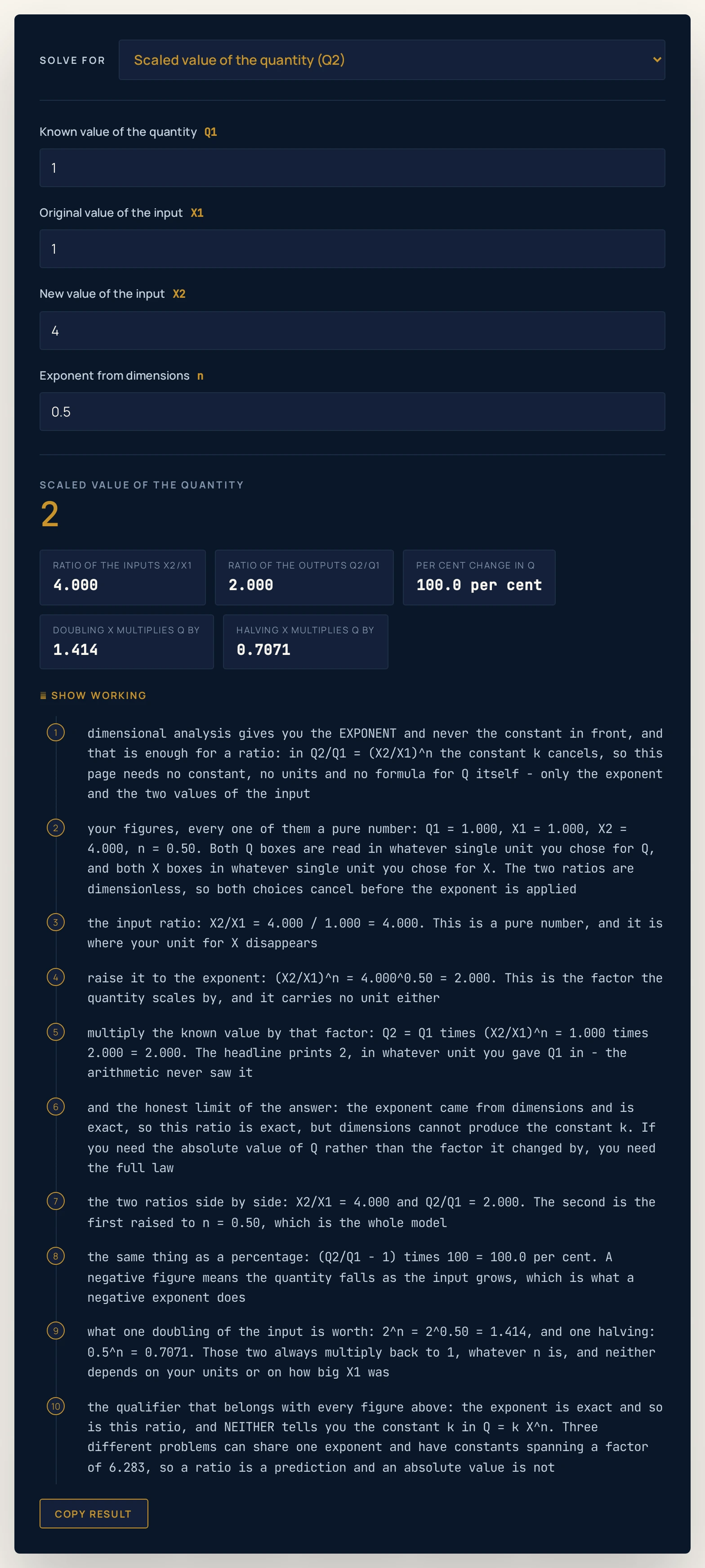
4.000, the output ratio 2.000, and no constant appears anywhere in the working — which is the only reason an exponent on its own is useful.Worked example: change one thing at a time
The table starts at the opening boxes, runs the three examples the page quotes, then moves the unknown through all four quantities on one single state, then changes the exponent and the input one at a time, and finally reaches the entries the calculator declines. Rows 4 to 7 are the important block: one set of numbers solved four ways, which is what a round trip through this relation looks like. Every answer and reading cell was read out of the running widget rather than worked out by hand, so where a cell and the tool ever part company, believe the tool.
| Step | Solving for | What you type | Headline answer | X2/X1 | Q2/Q1 | Per cent change | Doubling factor | Halving factor |
|---|---|---|---|---|---|---|---|---|
| The page as it opens | Q2 | Q1 1, X1 1, X2 4, n 0.5 | 2 | 4.000 | 2.000 | 100.0 per cent | 1.414 | 0.7071 |
| A satellite orbit six times higher | Q2 | Q1 1, X1 1, X2 6, n 1.5 | 14.7 | 6.000 | 14.70 | 1370 per cent | 2.828 | 0.3536 |
| The exponent behind a doubled radius | n | Q1 1, Q2 2.828, X1 1, X2 2 | 1.5 | 2.000 | 2.828 | 182.8 per cent | 2.828 | 0.3536 |
| The reference state, solved forwards | Q2 | Q1 1.419, X1 0.5, X2 2, n 0.5 | 2.838 | 4.000 | 2.000 | 100.0 per cent | 1.414 | 0.7071 |
| The same boxes, solved for the original | Q1 | Q2 2.838, X1 0.5, X2 2, n 0.5 | 1.419 | 4.000 | 2.000 | 100.0 per cent | 1.414 | 0.7071 |
| The same boxes, solved for the new input | X2 | Q1 1.419, Q2 2.838, X1 0.5, n 0.5 | 2 | 4.000 | 2.000 | 100.0 per cent | 1.414 | 0.7071 |
| The same boxes, solved for the exponent | n | Q1 1.419, Q2 2.838, X1 0.5, X2 2 | 0.5 | 4.000 | 2.000 | 100.0 per cent | 1.414 | 0.7071 |
| A quantity that does not scale | Q2 | Q1 5, X1 2, X2 7, n 0 | 5 | 3.500 | 1.000 | 0.000 per cent | 1.000 | 1.000 |
| Half the length instead of four times | Q2 | Q1 1, X1 1, X2 0.5, n 0.5 | 0.7071 | 0.5000 | 0.7071 | -29.29 per cent | 1.414 | 0.7071 |
| An inverse-square law at twice the distance | Q2 | Q1 1, X1 1, X2 2, n -2 | 0.25 | 2.000 | 0.2500 | -75.00 per cent | 0.2500 | 4.000 |
| Kinetic energy at three times the speed | Q2 | Q1 1, X1 1, X2 3, n 2 | 9 | 3.000 | 9.000 | 800.0 per cent | 4.000 | 0.2500 |
| The same scaling in milliseconds and centimetres | Q2 | Q1 1419, X1 50, X2 200, n 0.5 | 2838 | 4.000 | 2.000 | 100.0 per cent | 1.414 | 0.7071 |
| How much longer to double the period | X2 | Q1 1, Q2 2, X1 1, n 0.5 | 4 | 4.000 | 2.000 | 100.0 per cent | 1.414 | 0.7071 |
| The orbit exponent recovered from its preset | n | Q1 1, Q2 14.696938, X1 1, X2 6 | 1.5 | 6.000 | 14.70 | 1370 per cent | 2.828 | 0.3536 |
| A zero original input is declined | Q2 | X1 0 instead of 1 | no answer | - | - | - | - | - |
| A negative original input is declined | Q2 | X1 -1 instead of 1 | no answer | - | - | - | - | - |
| A zero new input is declined | Q2 | X2 0 instead of 4 | no answer | - | - | - | - | - |
| A zero known value is declined | Q2 | Q1 0 instead of 1 | no answer | - | - | - | - | - |
| A zero scaled value is declined | n | Q1 1, Q2 0, X1 1, X2 2 | no answer | - | - | - | - | - |
| Two equal inputs are declined in the exponent mode | n | Q1 1, Q2 2, X1 2, X2 2 | no answer | - | - | - | - | - |
| A zero exponent is declined in the new-input mode | X2 | Q1 1, Q2 2, X1 1, n 0 | no answer | - | - | - | - | - |
Rows 1 to 3 are the three questions this page exists for. Row 1 is the prediction: an exponent of 0.50 turns four times the length into 2.000 times the period. Row 2 is the same step with the orbital exponent 1.50, where six times the radius gives 14.70 times the period — a 1370 per cent increase from one line of arithmetic.
Row 3 runs it backwards and is the only direction that needs no theory at all. Two measurements, a doubled radius and a period 2.828 times longer, give n = 1.5. That is the exponent dimensional analysis predicts for an orbit, recovered from data, with the constant cancelling out of the calculation completely.
Rows 4 to 7 are one state solved four ways. The state is a pendulum lengthened from 0.5 to 2, entered as its printed period 1.419 fed forward, which the calculator turns into 2.838. Each row hands back four of those five boxes and asks for the fifth, and the answers come out 2.838, 1.419, 2 and 0.5 with the identical set of readings every time.
That is a tautology and it is worth saying so: one equation rearranged four ways can only disagree with itself in the last floating-point digit, and row 7's 0.5 comes back out of the same arithmetic that put 2.838 in. The pendulum's own period at a length of 2.000 m is 2.837 s, worked from the full small-amplitude law at that length with standard gravity, instead of scaled up from the printed 1.419. The ratio is exactly 2.000 either way, and that last-digit gap is why a rounded figure should never be fed into the next step — these rows do it deliberately, where it costs nothing and shows what it costs.
Rows 8, 10 and 11 change the exponent; row 9 changes the input instead. Row 8 is n = 0, which the calculator accepts: the output ratio is 1.000 and Q2 = Q1 exactly however far the input moves. That is not a degenerate case but a result — it is the dimensional statement that a pendulum's period does not depend on its mass.
Row 9 holds the exponent at 0.5 and moves the input the other way, while rows 10 and 11 run the exponent down to -2 and up to 2. Half the length gives 0.7071 of the period, exactly the halving factor from row 1's readings; an exponent of -2 gives 0.2500 and a -75.00 per cent change; and n = 2 turns three times the speed into 9.000 times the kinetic energy. The factor of one half in that law never appears, because a dimensionless factor cancels in the ratio.
Rows 12 to 14 are the units point and the design question. Row 12 types the whole of row 4 in milliseconds and centimetres instead of seconds and metres: 1419, 50 and 200 in place of 1.419, 0.5 and 2. Every reading is identical to row 4's, and only the headline changes — to 2838, which is the same fed-forward answer in the unit it was asked in.
Row 13 asks the design question instead: how much input do I need for twice the output? With n = 0.5 the answer is 4 times, which is the first row read from the other end. Row 14 recovers the orbital exponent from the preset's own eight-figure value and gets 1.5 rather than a near miss, which is what those extra digits are for.
Rows 15 to 21 sit outside the domain and are declined there rather than answered. A zero original input makes the ratio undefined and a negative one puts a negative base under a fractional exponent, which is not a real number. A zero known or scaled value makes every ratio zero or negative and leaves the exponent unrecoverable.
The last two are the ones worth understanding. Two equal inputs are refused only when the exponent is the unknown, because ln(X2/X1) is then ln(1) = 0; and a zero exponent is refused only when the new input is the unknown, because every X2 then gives the same output and there is nothing to solve. The same n = 0 that row 8 answers perfectly is declined in row 21, and that is the correct behaviour in both places.
Formula and symbol reference
One relation does all the work, and it is a division rather than a derivation. If a quantity obeys a power law Q = k X^n at two values of the input, dividing one statement by the other removes k entirely and leaves Q2/Q1 = (X2/X1)^n. Rearranged for each of the four unknowns that is Q2 = Q1 (X2/X1)^n, Q1 = Q2 / (X2/X1)^n, X2 = X1 (Q2/Q1)^(1/n) and n = ln(Q2/Q1) / ln(X2/X1) — the four positions of the Solve for menu.
The exponent itself comes from somewhere else, and that is the point of the method. Write the quantity you want as Q = k times each ingredient raised to an unknown power, demand that the exponents of mass, length and time match on both sides, and three base dimensions give you three linear equations. For a pendulum period from length, gravity and mass they read mass: 0, length: p + q = 0 and time: -2q = 1, so q = -0.50, p = 0.50 and the mass exponent is 0.00.
Dimensions stop there, and the stopping point is exact. The law is T = k L^0.50 g^-0.50, the exponent 0.50 is the number this calculator wants, and k is not something the method can produce: for a pendulum at small amplitude it happens to be 2*pi, which comes from solving the equation of motion, and the pendulum period formula guide is where that constant and its conditions belong. The same three rows run for an orbital period and give the exponent 1.50; squaring that statement is Kepler's third law, and the Kepler third law calculator is the tool for the version with its constant in place.
The reach of the method is not uniform, and three problems make that vivid. A pendulum period, a fall time from rest and the speed of a wave on a string all come out with the identical exponent triple, and their constants are 2*pi at small amplitude, the square root of two, and exactly 1. The first two are 6.283 and 1.414, a span of 6.283 across the three — so for the string the exponents are the whole answer, and for the pendulum they are a sixth of it.
| Symbol | Meaning | Unit | Values used on this page |
|---|---|---|---|
| Q1 | Known value of the quantity — the value of Q you already have, at the original input. A solve target | none: a pure number in your own unit | Opens on 1, which makes every answer read as a factor. Presets also use 5 and 1419. Must be positive. |
| Q2 | Scaled value of the quantity — the value of Q at the new input. The solve target the page opens on, and the only box with no default | none: a pure number in the same unit as Q1 | A result: 2.000 at the opening boxes, 14.70 for an orbit six times higher, 0.2500 for an inverse-square law at twice the distance. |
| X1 | Original value of the input — the value of X at which Q1 was measured. The one field that is never a solve target | none: a pure number in your own unit | Opens on 1. Presets also use 2 and 50. Must be positive: a negative base under a fractional exponent is not real. |
| X2 | New value of the input — the value of X you are asking about. A solve target, and the design question | none: a pure number in the same unit as X1 | Opens on 4, a pendulum four times as long. Presets reach 0.5, 2, 3, 6, 7 and 200. |
| n | Exponent from dimensions — the single power in the law, and what dimensional analysis actually gives you. A solve target, and the experimental direction | none: a pure number | Opens on 0.50. The exponents this cluster derives are 0.50, 1.50, 2.00, 1.00, -0.50, -1.00 and 0.00; the presets use 0.50, 1.50, 2.00, 0.00 and -2.00. |
| X2/X1 | Ratio of the inputs, the first reading. This is where your unit for X cancels | none: a pure number | A reading: 4.000 at the opening boxes, 3.500 for the quantity that does not scale, 0.5000 at half the length. |
| Q2/Q1 | Ratio of the outputs, the second reading. The input ratio raised to the exponent, and the whole model in one number | none: a pure number | A reading: 2.000 at the opening boxes, 9.000 for kinetic energy at three times the speed, 1.000 when the exponent is zero. |
| 2^n and 0.5^n | What one doubling and one halving of the input are worth, the last two readings. They always multiply back to 1 | none: pure numbers | A reading: 1.414 and 0.7071 at n = 0.50, 2.828 and 0.3536 at n = 1.50, 0.2500 and 4.000 at n = -2.00. |
The physics: why a ratio needs no constant
A power law written out in full has two unknowns in it: the exponent and the constant. Q = k X^n cannot be evaluated without both, which is why a dimensional result on its own looks like half an answer. Divide two instances of it, though, and k disappears exactly — not approximately, and not only for small changes.
That is the whole mechanism, and it is worth being precise about what survives it. The constant cancels, the units cancel, and any dimensionless factor cancels with them: a factor of one half, a whole number, even a function of a dimensionless group such as an angle, as long as it is the same in both instances. What is left is the exponent, and the exponent is the one thing dimensional analysis gives you exactly.
The same cancellation is why this page needs no unit menu, which is unusual for a calculator on this site. Unit conversion matters when you are comparing two quantities measured differently; here you are comparing a quantity with itself, so your unit appears in the numerator and the denominator of the same ratio and leaves no trace. The SI prefix converter is the tool for the conversion job proper — this one deliberately does not do it.
What the cancellation cannot do is turn a ratio into an absolute value, and the gap is larger than it looks. Load the pendulum four times as long preset and the answer is 2.000 times the period, which is exact. The actual period of a 0.5 metre pendulum is not in that number anywhere, and it cannot be got out of it: the exponent is exact, the prediction is exact, and neither tells you the constant. The pendulum period calculator is where that constant lives, with the small-amplitude condition attached to it.
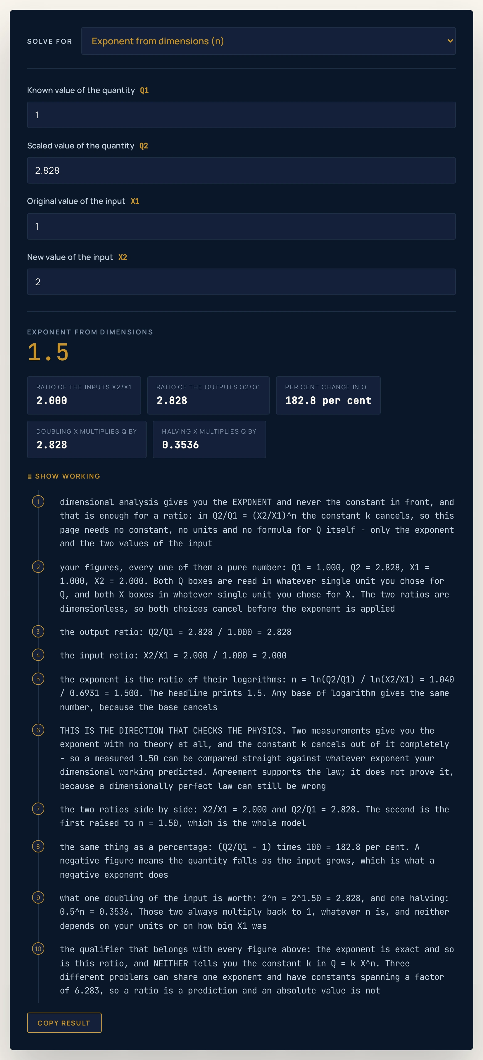
2.828 times longer give n = 1.5 — the orbital exponent recovered from two numbers, with the constant cancelling out of the calculation entirely.Where the dimensional analysis calculator breaks down
The arithmetic here is exact to the last digit a double can hold, and there is no physical constant in it to be uncertain about. What goes wrong is the modelling: an exponent that was never a dimensional result, a law that is not a power law at all, and a method that cannot see a factor.
- A matching exponent does not make a law correct
- This is the one place the page could ship something false, so the qualifier appears every time the claim does. Matching dimensions are necessary and not sufficient: the method is blind to any dimensionless factor, so
1/2 m v^2and2 m v^2have identical dimensions and the second is four times too big. The mechanics formulas guide states that conclusion about the unit check; this cluster is where it is measured in exponents. A ratio from this page is an exact statement about how a quantity changes, and nothing more. - The exponent has to be a real exponent, and the page cannot check it
- Type any number into the exponent box and the calculator will scale by it. It has no way of knowing whether
0.5came out of a dimensional matrix, out of a curve fit or out of a guess. Worse, homogeneity does not always pin the exponents down even when it is applied correctly: when the chosen ingredients are dimensionally dependent, several different exponent triples can all be perfectly homogeneous, and an independent reference written before this page existed exhibits three for one problem. - Not every relation is a power law
- The whole model assumes
Q = k X^nwith one constant exponent. An exponential, a logarithm, a sum of two power laws with different exponents, or a power law that changes exponent across a transition will all give a misleading answer here, and the warning sign is usually that the exponent you measure in one decade does not match the one you measure in the next. Solving fornat two different pairs of points is the cheapest test there is. - Three base dimensions are a choice, not the whole system
- This cluster works in mass, length and time, because that is what the mechanical quantities need. Electric charge, current, voltage and resistance need the electric-current dimension; temperature, entropy and specific heat need the thermodynamic-temperature one; amount of substance and molar mass need their own. That is not a limitation of the method — the same elimination runs in all seven base dimensions unchanged — but an exponent derived in three dimensions for a quantity that needs four is simply wrong.
- Dimensionless groups are a different subject, and this page is not it
- Counting how many independent dimensionless groups a problem has, and what to do with them, is the Buckingham pi theorem, and nothing here computes or implies any part of it. The same goes for dynamic similarity and for the named groups that come out of it: the Reynolds number guide is where that belongs. No figure for any of it appears anywhere on this page.
- Precision and uncertainty are not modelled
- The page prints four significant figures because that is the house ceiling, not because your inputs justify four. An exponent recovered from two noisy measurements inherits that noise, and nothing here propagates it: there is no error bar, no significant-figure arithmetic and no rounding advice. Two inputs carrying two figures cannot support a four-figure answer, however many digits the headline shows.
- A refusal is an answer, not a fault
- A zero or negative value in any of the four boxes a mode reads, two equal inputs when the exponent is the unknown, and a zero exponent when the new input is the unknown are all declined in words rather than answered with an infinity or a NaN. The two conditional ones are worth reading twice:
n = 0is a perfectly good input and is refused only as a route toX2, and equal inputs are fine in every mode except the one that takes their logarithm. - The calculator measures nothing — you supply the numbers
- Four numbers go in, one relation is rearranged, and the answer describes the power law you described. The preset names are shorthand for the five figures behind them, and the exponents in them are the ones a dimensional derivation produces for those problems; none of them is a measurement this page made.
Where dimensional scaling is actually used
- Turning a dimensional derivation into a number
- This is the forward question and the reason the page opens where it does. You have just worked out that a period goes as the square root of a length; the next thing anybody asks is what happens if the length quadruples, and the answer is
2.000times. Nothing about the constant is needed, which is the only reason an exponent on its own was worth deriving. - Checking a derived exponent against two measurements
- Point Solve for at the exponent and the page becomes an experimental check. Two values of the input, two values of the output, and the slope on a log-log plot comes back with the constant cancelled out. Agreement with what dimensions predicted is real evidence for the law; disagreement usually means an ingredient is missing from the derivation rather than that the arithmetic is wrong.
- Answering the design question backwards
- How long must the pendulum be to double the period? Point Solve for at the new value of the input, ask for an output ratio of 2, and the answer is
4times the length. This is the direction where a small exponent is expensive: atn = 0.50every doubling of the output costs a factor of four in the input, and atn = 0.25it would cost sixteen. - Seeing which ingredient does not matter at all
- An exponent of zero is a result, and it is often the most useful one. Load a quantity that does not scale and the output ratio reads
1.000while the input changes by3.500: the quantity simply does not respond. For a pendulum that is exactly what the mass exponent comes out as, which is why a heavy bob and a light one of the same length keep the same period. - Scaling an energy or a power with speed
- Kinetic energy goes as the square of the speed, so three times the speed is
9.000times the energy — and the factor of one half never enters the calculation. The kinetic energy calculator is the tool when you want the joules rather than the factor, and that is the one it carries the one half for. - Comparing a model across units without converting anything
- Because both ratios are dimensionless, you can hand this page figures in whatever units they arrived in, as long as each pair is internally consistent. The milliseconds and centimetres preset is the same physical scaling as the opening boxes typed in different units, and every reading beside the answer is identical. That is a property of the method rather than a convenience of the page.
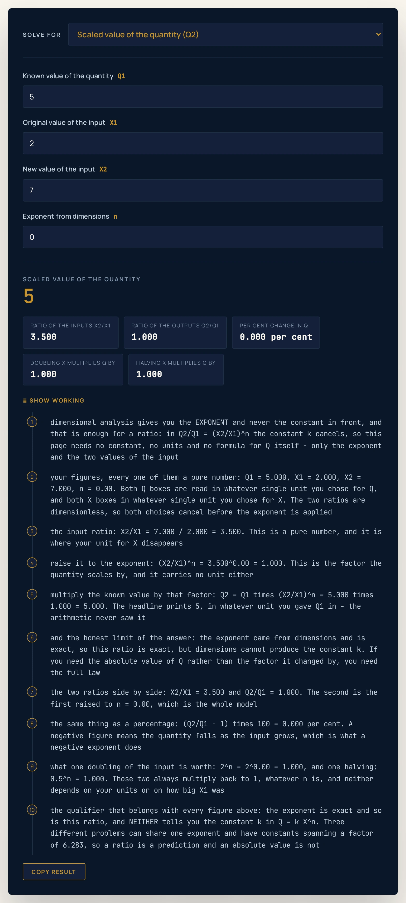
3.500 and the output ratio stays at 1.000, so the scaled value is 5 — the dimensional statement that this quantity does not depend on that input at all.Where to go next
For the method that produces the exponent — the exponent vectors, the three rows per problem, the residual that tells you which ingredient is wrong, and eight worked derivations — read the dimensional analysis guide, which this tool is the arithmetic half of. The SI units guide sets up the base quantities the exponents are counted over, and the physics formulas reference is the finished-laws counterpart to a page that only gives you their shape.
Three more posts pick up what this page leaves out. The pendulum period formula guide and the Kepler's laws guide carry the two constants dimensions cannot produce, and the problem-solving guide puts the dimensional check in its place as one step of a wider routine.
Four tools sit next to this one. The SI prefix converter handles the conversion job this page deliberately avoids; the Kepler third law calculator and the pendulum period calculator evaluate the two laws with their constants in place; and the kinetic energy calculator is the n = 2 case in full.
The full physics lab library and calculator index are open too.
Frequently asked questions
What does the dimensional analysis calculator work out?
It solves Q2 = Q1 (X2/X1)^n in all four directions: the scaled value of a quantity, the original value behind a scaled one, the new value of the input you would need for a given change, and the exponent itself. Beside the answer it prints the input ratio X2/X1, the output ratio Q2/Q1, the percentage change in Q, and what one doubling and one halving of the input are worth. The exponent is the number dimensional analysis gives you; the calculator is what you do with it once you have it.
Why do none of the boxes have a unit?
Because every quantity on the page is a pure number. X2/X1 is a ratio of two values of the same input, so whatever unit you measured X in cancels before the exponent is applied, and Q2/Q1 cancels your unit for Q in exactly the same way. Enter both Q values in one unit of your choosing and both X values in another, and the answer is identical: an independent check this cluster runs gets the same scaling factor to one part in a million million from seconds and metres as from milliseconds and centimetres. That is also why the page needs no conversion at all.
Where does the exponent n come from?
From dimensional analysis. Write the quantity you want as a constant times each ingredient raised to an unknown power, demand that the exponents of mass, length and time match on both sides, and you get three linear equations in three unknowns. For a pendulum period from length, gravity and mass the rows read mass 0, length p + q = 0 and time -2q = 1, so the length exponent is 0.50 and the mass drops out entirely. For an orbital period from radius and the gravitational parameter the same method gives 1.50.
Is n = 0 a valid entry?
Yes, and it is one of the most useful results the method produces. An exponent of zero means the quantity does not scale with that input at all, so Q2 = Q1 exactly however far you move X. The pendulum is the standard example: the mass exponent comes out as exactly zero, which is the dimensional statement that a heavy pendulum and a light one of the same length keep the same period. The calculator accepts it in three of its four directions and refuses it in one, because an exponent of zero leaves the new value of the input completely unconstrained.
Why will the calculator not accept a zero or negative input?
Because the model is a ratio of two positive values. An original input of zero makes X2/X1 undefined, and a negative value under a fractional exponent is not a real number: the square root of a negative length has no meaning as a period. A zero known value of the quantity makes every output ratio zero and leaves the exponent unrecoverable, and a zero scaled value does the same from the other end. In each case the page declines the entry in words rather than printing an infinity or a NaN.
Why does solving for the exponent need two different values of the input?
Because the exponent is the ratio of two logarithms, n = ln(Q2/Q1) / ln(X2/X1), and if X2 equals X1 the lower logarithm is ln(1) = 0. One input value tells you nothing about how the quantity responds to a change in it; two tell you the slope on a log-log plot, which is the exponent. That is the experimental direction of this page, and the constant in front cancels out of it completely.
Does a correct exponent mean the law is right?
No, and that is the one thing this page is most careful about. Matching exponents is necessary and not sufficient: a dimensionless factor is completely invisible to the method, so 1/2 m v squared and 2 m v squared have identical dimensions and the second one is four times too big. Three different problems can even share one exponent and have constants that span a factor of 6.283. A ratio from this page is an exact prediction about how a quantity changes; it is not a claim about the absolute value of anything.
Why does the headline read 2 when the working says 2.000?
They are the same number to four significant figures. The shared calculator engine formats the headline with trailing zeros dropped, so an answer of exactly two prints as 2, while the working and the readings keep the house four-figure form of 2.000. Nothing is rounded twice: each figure is formatted once from the full-precision value behind it. Where the worked table does feed a printed figure forward, at the 1.419 of rows 4 to 7 and the 1419 of row 12, the prose names it as a typed input and gives the 2.837 the full law returns in place of the 2.838 that route produces.
Can this calculator give me the constant in front of the law?
No, and no amount of dimensional reasoning can. For a pendulum at small amplitude the constant is 2*pi, for a fall from rest it is the square root of two, and for the speed of a wave on a string it is exactly 1 - three problems whose dimensional answer is the identical exponent triple. The constant comes from solving the actual equation of motion or from measurement, and the page links the guides that carry each one. What dimensions give you is the exponent, and that is what this page turns into a number.
What is deliberately not on this page?
There is no Buckingham pi theorem and no counting of dimensionless groups, no Reynolds number or dynamic similarity, no uncertainty propagation or significant-figure arithmetic, no SI prefix conversion, no base-unit definitions and no natural or Planck units. None of those is modelled here and no figure is given for any of them. The page solves one relation in four directions and stops, and the related guides pick up each of those subjects in its own place.
References & formula source
- The relation this page solves is the scaling form of a power law, Q2/Q1 = (X2/X1)^n. It follows from Q = k X^n by division, and the dimensionless constant k cancels exactly: an independent reference written before this page existed and sharing no code with it checks that against the exact formulas of six real power laws with their real constants over 1,200 random pairs and finds a worst relative discrepancy of 3.925e-16.
- The exponents this page takes as input come from dimensional homogeneity: any physically meaningful equation must have the same dimensions on both sides. Demanding that for a trial law gives one linear equation per base dimension, and in the three mechanical dimensions of mass, length and time that is a three-by-three system. Source: Wikipedia, "Dimensional analysis", for the homogeneity statement, for homogeneity as a plausibility check, and for the commensurable and incommensurable distinction. The same article is the source for the Buckingham pi theorem being a statement about the rank of the dimensional matrix, which this page does not cover.
- The method is necessary and not sufficient, and this page states that wherever it states a result. A dimensionless factor is invisible to it, so one half m v squared and two m v squared have identical dimensions while the second is four times too big; a dimensionally perfect equation can still be physically wrong; and when the chosen ingredients are dimensionally dependent, homogeneity does not even pin the exponents down to one answer. An independent reference written before this page existed exhibits three different exponent triples for one problem that are all perfectly homogeneous.
- The constants quoted on this page are not dimensional results and are named as such. For a pendulum the constant is 2*pi and only at SMALL AMPLITUDE: the fetched source states the condition as theta much less than 1 radian, often cited as less than 0.1 radians or about 6 degrees, with an approximation error of order theta cubed, and the independent reference measures the real period as 1.741 per cent above the small-angle value at 30 degrees from the series that source gives. Source: Wikipedia, "Pendulum (mechanics)". The pendulum law itself belongs to the pendulum period formula guide and the orbital law to the Kepler laws guide, both linked above.
- Three base dimensions are a choice, not the whole of the system. The International System of Quantities has seven base quantities, and the dimension of a quantity is written as a product of all seven raised to positive, negative or zero exponents; electric charge, current, voltage and resistance need the electric-current dimension, temperature and entropy need the thermodynamic-temperature one, and amount of substance needs its own. The elimination this page relies on runs in seven dimensions unchanged. Source: Wikipedia, "International System of Quantities".
- Not modelled anywhere on this page, and no figure is published or implied for any of it: the Buckingham pi theorem and the counting of dimensionless groups, Reynolds number and dynamic similarity, uncertainty propagation and significant figures, numeric unit conversion and the SI prefixes, natural, Planck or geometrised units, directed or anisotropic dimensions, and dimensional regularisation.
- Every figure quoted in the prose and the tables above is either a string this calculator printed for the inputs named beside it, or a figure from an independent reference written before this page existed, which runs 288 checks with 0 failures. A printed value is fed forward in one part of the table only and the prose says so: rows 4 to 7 and row 12 type the printed 1.419 back in, which is how they reach 2.838 where the full law gives 2.837. Where a table cell and the running widget ever part company, believe the widget.
- Further reading: Dimensional analysis — Wikipedia