Jerk in physics is the rate at which acceleration changes, the third derivative of position, measured in metres per second cubed. Because a constant acceleration has no jerk, the familiar displacement formula stops at the square of the time. Add a constant jerk and one more term appears: a sixth of the jerk times the time cubed.
Stand in a lift as it sets off. The unpleasant part is never the steady climb in the middle; it is the half second at the start, when the floor changes how hard it is pushing you. Ask a lift engineer what they tune to fix that and they will not say acceleration.
They tune how quickly the acceleration arrives. That rate has a name, a unit and a formula of its own — and it is also the reason one whole term goes missing from the displacement equation most students meet first.
What Is Jerk in Physics?
Jerk is the rate of change of acceleration, so it stands to acceleration exactly as acceleration stands to velocity.
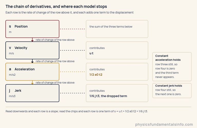
Think of the quantities as a chain of slopes. Velocity is the slope of a position–time graph, acceleration is the slope of a velocity–time graph, and jerk is the slope of an acceleration–time graph. Each step down the chain asks the same question of the row above it: how fast is this changing?
Its SI unit follows from that chain. Acceleration is measured in metres per second squared, so its rate of change is measured in metres per second cubed, m/s3. A jerk of 2 m/s3 means the acceleration is climbing by two metres per second squared every second.
Here is the part worth carrying away. You feel acceleration as apparent weight; you feel jerk as the moment that weight changes. The lurch as a driver comes off the brake, the settle at the top of a lift, the sideways kick as a train leaves a straight and enters a curve — each one is a jerk, not an acceleration.
Hold the acceleration steady and that sensation stops, however hard the push. Which is why comfort engineering is so often an argument about jerk and so rarely an argument about acceleration.
The Displacement Formula Under Constant Jerk
When the jerk is constant, the displacement over an interval takes one extra term beyond the constant-acceleration form.
Every symbol in it is something you already measure, with one addition:
- s — displacement over the interval, in metres (m).
- u — velocity at the start of the interval, in metres per second (m/s).
- a0 — acceleration at the start of the interval, in m/s2. This is the figure a constant-acceleration equation would use for the whole journey.
- j — the jerk, in m/s3, held constant across the interval.
- t — elapsed time, in seconds (s).
That subscript on a0 is doing real work. Once the acceleration is ramping there is no single value of it, so a figure quoted without saying when it was taken is ambiguous: it is a0 at the start, a0 + j t at the end, and a0 + 1/2 j t on average across the interval.
Rearranged, the same relation hands back any one of the four unknowns from the other three, and the jerk physics calculator runs all four modes with the dropped term printed beside each answer. The elapsed time is the exception. It enters as a cube, and a cubic can have three real roots with no honest way to choose between them, so it stays an input.
One sentence of orientation before going further. The five SUVAT equations, their symbol table and the rule that picks between them are covered in full elsewhere on this site and none of it is repeated here; this page begins at the line where that rule stops, the one that says the acceleration must be constant.
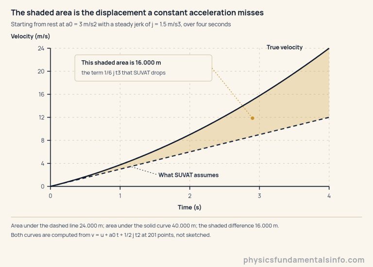
Below, the lab draws a velocity–time graph for whatever you dial in. The dashed line is the velocity a constant acceleration assumes, the solid curve is the truth, and the region between them is the displacement at issue. One caution about reading it: the vertical scale resizes itself to fit whatever is on screen, so the band’s width in pixels is a ratio rather than a size. Watch whether a band appears at all and which side of the dashed line the curve runs on; take the metres from the readouts, which change as you drag.
Those three terms are not arbitrary, and the diagram below says where each of them comes from. Read the chain downwards and every row is the slope of the row above; read the chips on the right and every row contributes one term to the displacement.
Five Displacement Formulas, and the One That Survives
Faced with an acceleration that will not sit still, most people reach for one of five expressions, and exactly one of them is exact.
Take a concrete case so the argument cannot hide. A body starts from rest, u = 0, with an initial acceleration of 3.000 m/s2 and a steady jerk of 1.500 m/s3, over 4.00 s. The true displacement is 40.000 m. Here is what each candidate returns.
| Method | Expression | Error against the truth | Exact | The worked case |
|---|---|---|---|---|
| SUVAT, acceleration taken at the start | u t + 1/2 a0 t2 | short by exactly 1/6 j t3 | No | 24.000 m, short by 16.000 m |
| SUVAT, acceleration taken at the end | u t + 1/2 (a0 + j t) t2 | long by exactly 1/3 j t3 | No | 72.000 m, long by 32.000 m |
| SUVAT, mean acceleration across the interval | u t + 1/2 (a0 + 1/2 j t) t2 | long by exactly 1/12 j t3 | No | 48.000 m, long by 8.000 m |
| Half the sum of the end velocities | 1/2 (u + v) t | long by exactly 1/12 j t3 | No | 48.000 m, long by 8.000 m |
| Simpson on the velocity–time area | (t/6)[v(0) + 4 v(t/2) + v(t)] | none | Yes | 40.000 m, the truth |
Read the error column first, because it is the point of the table. Every miss is an exact multiple of j t3 — not an estimate, not a fudge factor — and the multiples are 1/6, 1/3, 1/12 and 1/12.
Measured in units of 1/12 j t3, those three SUVAT errors come out at -2, +4 and +1 for the start, end and mean accelerations. So the repair that looks most careful, taking the acceleration at the end of the interval, is four times the size of the mean-acceleration error and twice the size of the start-acceleration one — and unlike that one, it overshoots rather than falling short.
Now the uncomfortable one. The expression s = 1/2 (u + v) t looks less like a model than like a definition: average the two end velocities, multiply by the time. It is the same expression as SUVAT fed the mean acceleration — problem 6 does that algebra line by line — and both run long by exactly 1/12 j t3. Their agreeing with each other settles nothing: it is a single expression written out twice.
What survives is the oldest idea of the five. The displacement is the area under the velocity–time graph, which our guide to motion graphs already teaches, and that method does not break here. What breaks is the trapezium, the straight-line shortcut normally used to evaluate it.
A trapezium measures the area beneath a straight chord. Ramp the acceleration and the velocity line bows into a parabola, so the chord encloses area the motion never had. Simpson’s rule weights the start, the midpoint and the end in the proportion 1 : 4 : 1, and that combination measures a parabola exactly.
Set the jerk to zero and every row of that table collapses onto the same answer. That is a definition rather than a discovery: with no jerk there is no third term, and the five expressions were never in disagreement in the first place.
Why the Gap Grows as the Cube of the Time
The term a constant acceleration drops grows as the cube of the elapsed time, so doubling the interval multiplies it by exactly eight.
Set the three terms beside each other and their exponents do the arguing. The velocity term grows as t, the acceleration term as t2, and the dropped jerk term as t3. Over a short interval the third is a rounding error. Over a long one it can be the largest of the three.
That is the honest answer to “does a small jerk matter?” — it depends entirely on how long you let it run.
Put all three terms on log axes and each becomes a straight line whose slope is its power of the time. Two things show up at once: the dropped term is the steepest line on the chart, and there are moments when it overtakes each of the others.
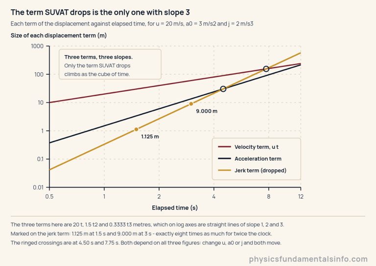
Those crossings have exact times. Setting the jerk term equal to the acceleration term, and then to the velocity term, gives two clean results:
Both are exact algebra. Neither is a constant of nature, and that distinction matters more than the formulas do. Each crossing time depends on the other two figures you started with, so there is no such thing as “the time when SUVAT stops working” — only the time at which, for these numbers, two terms happen to be equal. Problem 8 works two of them out.
Real-World Examples of Jerk
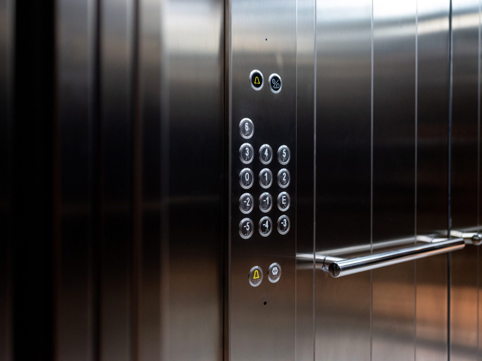
Lift ride quality. Comfort in a lift is governed by how quickly the acceleration arrives rather than by how large it becomes. On the figures collected in Wikipedia’s article on jerk, most passengers are reported to rate a vertical jerk of 2 m/s3 as acceptable and 6 m/s3 as intolerable, and 0.7 m/s3 is the recommended limit for hospitals.
Those are rated jerks, not ride profiles, and the difference is worth spelling out. Hold 6 m/s3 for a full two seconds and the car reaches 12 m/s2 and 12 m/s — roughly 43 km/h, straight up. No lift in service does that. A real one ramps its acceleration for a fraction of a second and then holds it steady, which makes the jerk zero for most of the ride.
Nor is there a standard that sets a limit. ISO 8100-34 specifies how lift ride quality is to be measured with respect to jerk, acceleration, vibration and noise, and explicitly does not specify acceptable or unacceptable levels. The three figures above are reported passenger ratings and a recommendation, which is a weaker and more honest thing than a standard.
Transition curves on rail and road. A curve that begins abruptly forces a step change in sideways acceleration, so alignments use a transition whose curvature builds gradually instead. Published design standards for high-speed rail run from 0.2 to 0.6 m/s3.
Read that range carefully, because it is not the same quantity as the lift figures. It is a lateral jerk, produced by the track’s curvature changing underneath the train, across the direction of travel rather than along it. The model on this page runs along one line, so those numbers belong in the conversation as the magnitude engineers design to and not in its jerk slot.
Roller coasters. Entering a loop, acceleration values can reach around 4g, about 40 m/s2, and riding in that environment is only possible because the track transitions into it. Notice what that figure is: an acceleration, not a jerk. The transitions exist to govern how quickly it arrives.
Motion control. Passenger lifts and machining tools are the classic motion-control applications, and the design goal in both is to make a transition as short as possible without exceeding the speed, acceleration or jerk limits set for it. Jerk gets a limit of its own there because it is the quantity considered whenever vibration is a concern.
One thread runs through all four. Nobody in those trades is arguing about how big the acceleration is allowed to be. They are arguing about how fast it is allowed to change.
Common Misconceptions About Jerk
“Jerk is just a violent acceleration.” It is a different quantity with a different unit. Hold a body at a large but perfectly steady acceleration and its jerk is zero, however punishing the ride feels. The 40 m/s2 a coaster reaches in a loop is an acceleration figure for the same reason, and quoting it as a jerk is a unit error rather than an exaggeration.
“SUVAT is wrong when the acceleration changes.” SUVAT is not wrong. It is exact, and it states its own condition plainly: the acceleration must be constant. Handing it a ramping acceleration is not a flaw in the equation but a question it was never asked, and the size of the resulting miss is predictable to the metre.
“s = 1/2 (u + v) t is a definition, so it always holds.” Averaging the two end velocities is only the same as averaging over the whole interval when the velocity changes at a steady rate. Ramp the acceleration and the velocity curve bulges, the two averages part company, and the formula runs long by exactly 1/12 j t3.
“A small jerk can be ignored.” Over a short interval, usually. The trouble is that the term it produces grows as the cube of the time while the terms SUVAT keeps grow as t and t2, so the question is never “is the jerk small?” but “small compared with what, over how long?”. A common student slip is to decide that once and reuse the decision on a much longer interval.
How Jerk Fits With SUVAT, Motion Graphs and Displacement
Jerk does not replace anything already on this site. It extends exactly one line of it, and leaves the rest standing.
Start with what is being measured. Everything here is a displacement along a single line, signed rather than a distance travelled, so a body that goes out and comes back can honestly return a small answer. The curve the lab draws is a velocity for the same reason: it carries a sign, and a negative jerk drags it down rather than reversing anything.
The bridge to motion graphs is the one worth drawing twice. That guide teaches slope going one way and area going the other, and both survive intact here. The only casualty is the trapezium, which is an arithmetic shortcut for the area rather than part of the rule.
And the SUVAT equations remain the right tool the moment the acceleration holds still, which it does far more often than not. This page is the neighbouring case, not a replacement, and the SUVAT calculator is still the faster route whenever that condition is met.
If you would rather watch the shape than read about it, the jerk physics simulator is that same lab on a page of its own, with worked cases to load and a caption that changes when the two curves merge into one line.
Where the Constant-Jerk Model Breaks Down
Constant jerk is an idealisation, in precisely the way constant acceleration is an idealisation.
Real motion has a jerk that changes too, and the series does not stop at the third term. The next one carries the fourth derivative of position with a 1/24 in front of it, and the one after that a 1/120. This page is the next term after constant acceleration, not the last word on the subject.
The practical fix for everything else has not changed either. Where an acceleration shifts in steps, or in any way that is not a steady ramp, the right answer is to break the motion into stages that each hold their own acceleration and run them in sequence. OpenStax’s College Physics states that assumption and that remedy explicitly, and nothing here overturns it. The closed form above removes the need for splitting in one case only: when the acceleration ramps at a steady rate.
Two more limits are worth naming. The model runs in one dimension, so a motion that also turns has a jerk with components this page cannot express. And the figures it quotes are rounded to three decimals while the arithmetic behind them is not, so three terms read off a screen need not add to the fourth in their last digit.
A last word on evidence. The simulator, the calculator and this page all run the same relation, so their agreeing with one another says nothing whatever about the world — only that one piece of algebra was implemented three times. The claims worth testing are the ones you can check against a real motion, and those come with a stopwatch rather than a screen.