A velocity–time graph is a straight line only while the acceleration holds still. Let the acceleration ramp instead — at a steady jerk, j = da/dt — and the line becomes a parabola, which is what this lab draws: the straight line a constant-acceleration equation assumes, the curve that actually happens, and the shaded band between them whose area is the displacement the straight line misses, 1/6 j t3. Four sliders set the initial velocity, the initial acceleration, the jerk and the clock, and four cards keep score.
Jerk in Physics: the Displacement SUVAT Cannot See
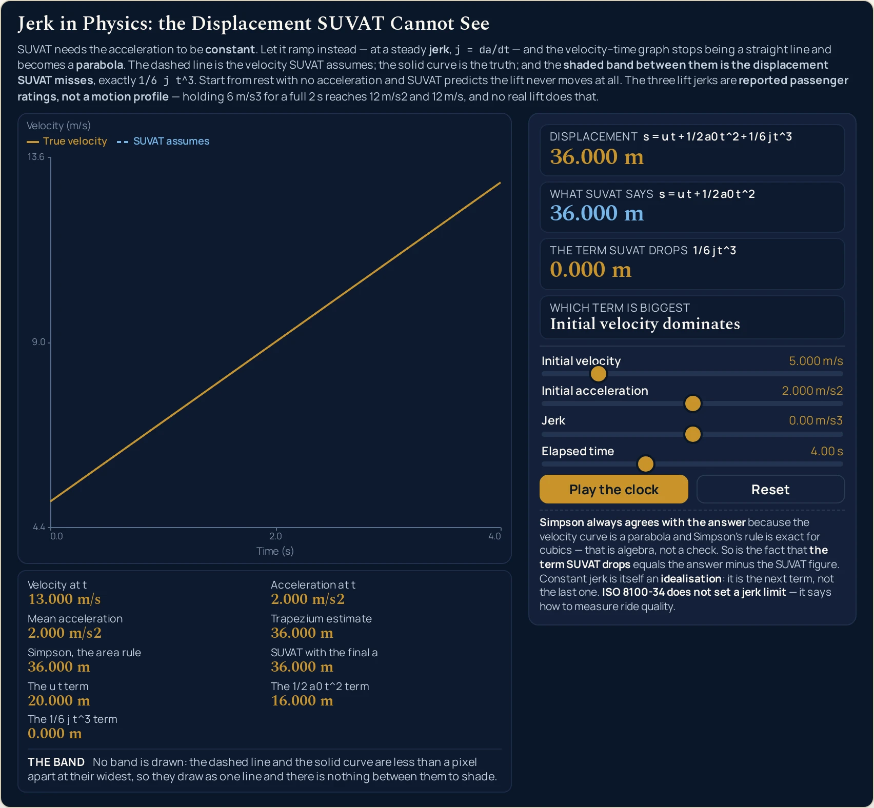
SUVAT needs the acceleration to be constant. Let it ramp instead — at a steady jerk, j = da/dt — and the velocity–time graph stops being a straight line and becomes a parabola. The dashed line is the velocity SUVAT assumes; the solid curve is the truth; and the shaded band between them is the displacement SUVAT misses, exactly 1/6 j t^3. Start from rest with no acceleration and SUVAT predicts the lift never moves at all. The three lift jerks are reported passenger ratings, not a motion profile — holding 6 m/s3 for a full 2 s reaches 12 m/s2 and 12 m/s, and no real lift does that.
Velocity at t4.000 m/s
Acceleration at t4.000 m/s2
Mean acceleration2.000 m/s2
Trapezium estimate4.000 m
Simpson, the area rule2.667 m
SUVAT with the final a8.000 m
The u t term0.000 m
The 1/2 a0 t^2 term0.000 m
The 1/6 j t^3 term2.667 m
The bandThe shaded band between the dashed line and the solid curve is the displacement SUVAT misses: the solid curve runs above the dashed line the whole way, so the straight-line answer is short by 2.667 m.
Displacement s = u t + 1/2 a0 t^2 + 1/6 j t^3
2.667 m
What SUVAT says s = u t + 1/2 a0 t^2
0.000 m
The term SUVAT drops 1/6 j t^3
2.667 m
Which term is biggest
Jerk dominates
Initial velocity0.000 m/s
Initial acceleration0.000 m/s2
Jerk2.00 m/s3
Elapsed time2.00 s
Simpson always agrees with the answer because the velocity curve is a parabola and Simpson's rule is exact for cubics — that is algebra, not a check. So is the fact that the term SUVAT drops equals the answer minus the SUVAT figure. Constant jerk is itself an idealisation: it is the next term, not the last one. ISO 8100-34 does not set a jerk limit — it says how to measure ride quality.
Load a real case on the sliders
Each button presses the lab’s own Reset and then writes all four sliders, so every load starts from the same place and a running clock is stopped before the new values land. Work down the list and watch What SUVAT says and Displacement disagree by more on some cases than on others. The three lift cases are named plainly because their jerk is a published figure; the rest carry -like, for reasons set out under the limits below.
Pick a case above, or drag the four sliders yourself.
What Is the Jerk Physics Simulator?
The jerk physics simulator is a free interactive physics lab that runs in your browser, with nothing to install and no sign-up. It plots velocity against time over one interval of motion: a dashed straight line for the velocity a constant-acceleration equation assumes, a solid curve for the true velocity when the acceleration ramps at a steady jerk, and a shaded band between the two whose area is the displacement the straight-line answer misses.
Four sliders set the initial velocity from 0 to 30 m/s, the initial acceleration from -6 to 10 m/s2, the jerk from -8 to 8 m/s3 and the elapsed time from 0 to 12 s, which is also the right-hand edge of the plot.
Four cards answer with the displacement s = u t + 1/2 a0 t2 + 1/6 j t3, what a constant-acceleration equation would have said, the term that equation drops, and one of four phrases naming which of the three terms is biggest.
Nine smaller cells carry the velocity and the acceleration at the elapsed time, the mean acceleration, the trapezium and Simpson estimates, the constant-acceleration answer taken at the final acceleration instead, and the three terms separately, with a sentence strip headed The band describing what the shading shows. Play the clock runs the elapsed time forward; Reset restores 0 m/s, 0 m/s2, 2 m/s3 and 2 s.
| Control | Range | Step |
|---|---|---|
| Initial velocity | 0 to 30 m/s | 0.5 m/s |
| Initial acceleration | -6 to 10 m/s2 | 0.2 m/s2 |
| Jerk | -8 to 8 m/s3 | 0.1 m/s3 |
| Elapsed time | 0 to 12 s | 0.1 s |
How to use the jerk in physics simulator
- Start from the state it opens in. The lab boots at rest on 0.000 m/s, 0.000 m/s2, 2.00 m/s3 and 2.00 s, with Displacement already reading 2.667 m and What SUVAT says 0.000 m. Reset returns all four sliders to exactly that and stops the clock if it is running.
- Set the initial velocity. Initial velocity runs from 0 to 30 m/s in steps of 0.5 and moves both curves by the same amount, because it is where each of them starts, so the vertical axis simply re-labels itself and the drawing does not change. It is one of two sliders — the other is Initial acceleration — that leave The term SUVAT drops exactly where it is: at either end it still reads 2.667 m.
- Set the initial acceleration. Initial acceleration runs from −6 to 10 m/s2 in steps of 0.2 and tilts the dashed line, which is the velocity the SUVAT equations assume all the way across. Take it to 10.000 m/s2 and the dropped term does not move either.
- Set the jerk. Jerk runs from −8 to 8 m/s3 in steps of 0.1 and is what bends the solid curve away from that line. Positive values put the curve above the dashed line and negative ones put it below, which flips the sign of The term SUVAT drops.
- Move the clock. Elapsed time runs from 0 to 12 s in steps of 0.1 and is both the length of the interval and the right-hand edge of the plot. It is the slider with the most leverage, because the dropped term grows as its cube.
- Read the four cards down the right. Displacement carries its own formula line,
s = u t + 1/2 a0 t2 + 1/6 j t3; What SUVAT says drops the last term; The term SUVAT drops is that term on its own; and Which term is biggest prints one of exactly four phrases, from Nothing has moved yet to Jerk dominates. - Read the nine cells under the graph. Velocity at t and Acceleration at t give the end of the interval, Mean acceleration the average across it, then three rival answers — Trapezium estimate, Simpson, the area rule and SUVAT with the final a — and finally the three terms separately.
- Read the strip headed The band. It describes the shading in words, names which curve is on top and says whether the straight-line answer is short or long, in metres. When there is nothing left to shade it says that instead of describing a gap you cannot see.
- Press Play the clock to let it run. Elapsed time then advances at 1.2 s of clock per second of real time and the button becomes Pause the clock; the other three sliders stay exactly where you put them. Past 12.00 s the clock returns to the start and runs the same case again.
If the acceleration in your problem really does hold still, this is more lab than you need. The SUVAT equations lab draws that case with a single acceleration slider and all five equations beside it, and the straight dashed line here is the line it draws. Come back the moment the acceleration starts changing.
Worked example: change one thing at a time
Every row below is one of the six preset buttons, and every cell is a string the running lab printed there. The first three hold the initial velocity, the initial acceleration and the clock still and move only the jerk; the last three add a starting velocity or a starting acceleration, and two of them turn the sign around. Where a cell and the lab ever part company, believe the lab.
| Preset | Sliders, as the panel reads them | Displacement | What SUVAT says | The term SUVAT drops | Which term is biggest |
|---|---|---|---|---|---|
| Lift, acceptable jerk | 0.000 m/s · 0.000 m/s2 · 2.00 m/s3 · 2.00 s | 2.667 m | 0.000 m | 2.667 m | Jerk dominates |
| Lift, hospital limit | 0.000 m/s · 0.000 m/s2 · 0.70 m/s3 · 2.00 s | 0.933 m | 0.000 m | 0.933 m | Jerk dominates |
| Lift, intolerable jerk | 0.000 m/s · 0.000 m/s2 · 6.00 m/s3 · 2.00 s | 8.000 m | 0.000 m | 8.000 m | Jerk dominates |
| Car pulling away-like | 0.000 m/s · 3.000 m/s2 · 1.50 m/s3 · 4.00 s | 40.000 m | 24.000 m | 16.000 m | Acceleration dominates |
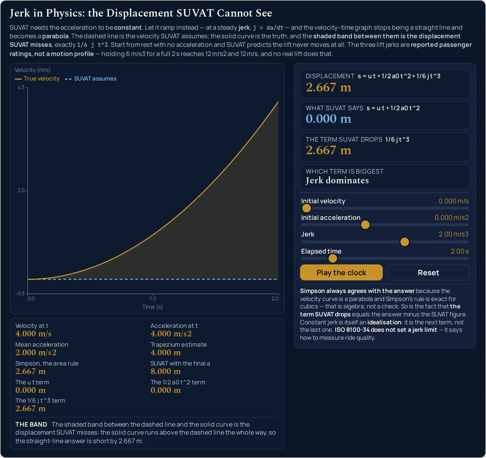
| Braking to a stop-like | 20.000 m/s · −2.000 m/s2 · −1.00 m/s3 · 4.00 s | 53.333 m | 64.000 m | −10.667 m | Initial velocity dominates |
| Ramp onto a cruise-like | 5.000 m/s · 2.000 m/s2 · −0.50 m/s3 · 4.00 s | 30.667 m | 36.000 m | −5.333 m | Initial velocity dominates |
Rows 1 to 3 are the whole lesson. All three begin from rest with no acceleration, so both of the quantities What SUVAT says is built from are zero and it prints 0.000 m every time. The lift has meanwhile risen 2.667 m at the acceptable figure, 0.933 m at the hospital one and 8.000 m at the intolerable one. Say that in metres and stop there: there is no percentage to take, because the figure you would divide by is zero.
Those three rows share a velocity, an acceleration and a clock, so the only thing separating them is the jerk, and the displacement follows it in proportion. That is the third term restated rather than a discovery, and it is worth noticing only because it makes the term’s job obvious. Velocity at t moves with it, in that same row order: 4.000, 1.400 and 12.000 m/s.
Those rows are what the model says at a published jerk, not a description of a lift. Hold 6.00 m/s3 for the full 2.00 s and the lab prints Acceleration at t 12.000 m/s2 and Velocity at t 12.000 m/s, about forty-three kilometres an hour straight up. Nothing in service does that: a real lift ramps for a fraction of a second and then holds its acceleration steady, with the jerk back at zero.
Rows 5 and 6 carry the other sign. A negative jerk bends the solid curve below the dashed line, so the straight-line answer overshoots and The term SUVAT drops comes out negative: −10.667 m and −5.333 m. The strip headed The band changes with it, saying the answer is long by that many metres rather than short by them.
Row 4 is worth a second look, because the card is not a warning light. Which term is biggest reads Acceleration dominates while the straight-line answer is still 16.000 m short of 40.000 m. The card ranks the three terms; it does not judge whether dropping one of them matters to you. If you want those figures to more places, or the same relation run backwards, the jerk physics calculator takes typed input and solves for any of the four quantities.
Formula and symbol reference
The lab works from one relation, s = u t + 1/2 a0 t2 + 1/6 j t3, with the velocity behind it v = u + a0 t + 1/2 j t2. Everything on the panel is one of those two read at a particular moment, or one of their three terms taken on its own.
The three terms grow at three different rates, and that is the only thing you need to keep in mind while dragging. The first is proportional to the clock, the second to its square and the third to its cube, so which of them matters depends entirely on how long an interval you asked about.
| Symbol | Meaning | SI unit | In this lab |
|---|---|---|---|
| s | Displacement over the whole interval, and the headline card. The area under the solid curve, which is not the area under the dashed one | metre, m | Three decimal places at every size, with no magnitude switch: “2.667 m” after Reset, “0.000 m” with the clock at 0.00 s, and “3384.000 m” with all four sliders at their top stops. |
| u | Initial velocity: how fast the body was already moving when the clock started. Where both curves begin on the vertical axis | metre per second, m/s | 0 to 30 in steps of 0.5, printed to three decimals: “0.000 m/s” after Reset and “30.000 m/s” at the top stop. Moving it alone never changes The term SUVAT drops, which still reads 2.667 m at either end. |
| a0 | Initial acceleration, the value at the very start of the interval. The slope of the dashed line, and the single figure a constant-acceleration equation would use throughout | metre per second squared, m/s2 | −6 to 10 in steps of 0.2: “−6.000 m/s2” at the bottom stop, “0.000 m/s2” after Reset, “10.000 m/s2” at the top. It leaves the dropped term at 2.667 m as well. |
| j | Jerk: how fast that acceleration is itself changing. The curvature of the solid line, and one of only two sliders that moves the dropped term | metre per second cubed, m/s3 | −8 to 8 in steps of 0.1, printed to two decimals: “2.00 m/s3” after Reset. The step is a tenth so that 0.70, 2.00 and 6.00 all land exactly on the grid; taken to “−8.00 m/s3” the dropped term reads −10.667 m. |
| t | Elapsed time, which is both the length of the interval and the right-hand edge of the plot | second, s | 0 to 12 in steps of 0.1, printed to two decimals: “2.00 s” after Reset. Left on the opening jerk and dragged to “12.00 s”, the displacement goes from 2.667 m to 576.000 m. |
| v at t | The true final velocity, printed as Velocity at t. The right-hand end of the solid curve | metre per second, m/s | “4.000 m/s” after Reset; 1.400, 4.000 and 12.000 m/s across the three lift cases; “726.000 m/s” with every slider at its top stop. |
| a at t | The acceleration at the end of the interval, printed as Acceleration at t. The slope of the solid curve where it stops | metre per second squared, m/s2 | “4.000 m/s2” after Reset, and exactly “0.000 m/s2” on the cruise-like ramp at 4.00 s, where a starting 2.000 m/s2 and a jerk of −0.50 m/s3 have just cancelled. |
| a mean | Mean acceleration over the interval, printed as Mean acceleration. Feeding this to a constant-acceleration equation gives the trapezium figure, not the truth | metre per second squared, m/s2 | “2.000 m/s2” after Reset, “6.000 m/s2” on the car-like case and “−4.000 m/s2” on the braking-like one. |
| u t | The velocity term, printed as The u t term. It grows in simple proportion to the clock | metre, m | “0.000 m” on all three lift cases, “80.000 m” on the braking-like case and “20.000 m” on the cruise-like ramp. |
| 1/2 a0 t^2 | The acceleration term, printed as The 1/2 a0 t^2 term. It grows as the square of the clock | metre, m | “0.000 m” on the lift cases, “24.000 m” on the car-like case and “−16.000 m” on the braking-like one. |
| 1/6 j t^3 | The jerk term, printed twice: as The term SUVAT drops among the cards and as The 1/6 j t^3 term among the cells. It grows as the cube of the clock | metre, m | “2.667 m” after Reset, “−10.667 m” on the braking-like case, “432.000 m” for the car-like ramp taken out to 12.00 s. |
| s trapezium | Half the sum of the starting and finishing velocities, times the clock, printed as Trapezium estimate. The straight-line area of a curved region | metre, m | “4.000 m” after Reset against a true 2.667 m, and “48.000 m” on the car-like case against 40.000 m. |
| s Simpson | The area rule with a parabola fitted through three points, printed as Simpson, the area rule | metre, m | Always the same string as the Displacement card: “2.667 m” after Reset, “40.000 m” on the car-like case. That agreement is algebra, not a check. |
| s final a | A constant-acceleration equation fed the acceleration measured at the END of the interval, printed as SUVAT with the final a. The repair that overshoots | metre, m | “8.000 m” after Reset against a true 2.667 m, and “72.000 m” on the car-like case against 40.000 m. |
Two rows there are easy to misread. Mean acceleration looks like the safe figure to quote and is not: feeding it to a constant-acceleration equation reproduces the Trapezium estimate exactly, and that cell reads 4.000 m on the opening state against a true 2.667 m. And Simpson, the area rule prints the same string as Displacement at every setting, which is a property of the arithmetic rather than evidence about it.
The physics: why a straight line cannot measure a curved area
The displacement over an interval is the area under the velocity–time graph, and that is true whatever the acceleration does. What changes when the acceleration ramps is the shape of the graph: the dashed line here is the one Motion Graphs in Physics draws for a constant acceleration, and the solid curve is a parabola sitting above or below it.
The area rule is not what breaks. The trapezium shortcut for evaluating it is, because a trapezium measures the area under a straight line and there is a curve there instead. The motion graphs lab is the place to watch the straight version before this one bends it, and the two labs draw the same axes on purpose.
The band is the difference between those two areas, and its size is 1/6 j t3. Leave the car-like case loaded and walk Elapsed time along: The term SUVAT drops reads 0.250 m at 1.00 s, 2.000 m at 2.00 s, 16.000 m at 4.00 s and 128.000 m at 8.00 s. Each doubling of the clock multiplies it by exactly eight; take the same case to 12.00 s and it reads 432.000 m, twenty-seven times its value at 4.00 s.
That cubic growth is why a constant acceleration is harmless over a short interval and dangerous over a long one. The two terms it keeps grow as the clock and as its square, so the term it drops starts small and then overtakes both. The card labelled Which term is biggest is watching exactly that race.
There is an exact moment when the dropped term catches each of the others, and you can park the sliders on it. With Initial acceleration at 3.000 m/s2 and Jerk at 1.50 m/s3, the clock at 6.00 s gives The 1/2 a0 t^2 term and The 1/6 j t^3 term both reading 54.000 m. One stop earlier they are 52.215 m and 51.345 m; one stop later, 55.815 m and 56.745 m, and the card has turned over to Jerk dominates.
The companion crossover is with the velocity term. Set Initial velocity to 1.500 m/s, Initial acceleration to 0.000 m/s2 and Jerk to 1.00 m/s3, and at 3.00 s The u t term and The 1/6 j t^3 term both read 4.500 m. Neither of these moments is a universal constant: each depends on the other two sliders, so there is no such number as the time when a constant acceleration stops working.
What the picture can tell you, and what it cannot. The vertical axis rescales at every setting to hold both curves, so the band’s width on screen is a ratio and not a size. Two settings can therefore shade the same width and carry very different answers. Read which curve is on top and whether a band is shaded at all, and watch The term SUVAT drops change as you drag; take every magnitude off the cards.
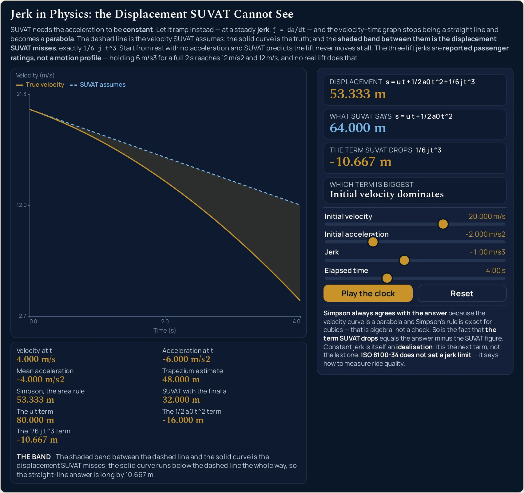
The shading switches off by a pixel test, not by a physics test. Once the two curves are less than one pixel apart at their widest separation on the plot as drawn, no band is shaded and the strip says so. The table below walks the jerk down at the opening state and then adds two settings where the band vanishes for a different reason.
| Setting | Displacement | What SUVAT says | The term SUVAT drops | The band |
|---|---|---|---|---|
| Opening state, jerk 2.00 m/s3 | 2.667 m | 0.000 m | 2.667 m | drawn |
| Opening state, jerk 0.50 m/s3 | 0.667 m | 0.000 m | 0.667 m | drawn |
| Opening state, jerk 0.30 m/s3 | 0.400 m | 0.000 m | 0.400 m | drawn |
| Opening state, jerk 0.10 m/s3 | 0.133 m | 0.000 m | 0.133 m | drawn |
| Opening state, jerk 0.00 m/s3 | 0.000 m | 0.000 m | 0.000 m | not drawn |
| Cruise-like ramp, jerk −0.50 m/s3, clock 0.10 s | 0.510 m | 0.510 m | 0.000 m | not drawn |
| Cruise-like ramp, jerk 0.00 m/s3, clock 4.00 s | 36.000 m | 36.000 m | 0.000 m | not drawn |
The 0.00 m/s3 row is the honest zero: the two curves are the same line, all three cards read 0.000 m and there is genuinely nothing between them to shade. The rows beneath 0.50 m/s3 are the only region where the shading narrows as the jerk comes down, because the vertical axis has reached its legibility floor and has stopped rescaling with it.
Above that floor the drawing does not change at all. At this state every jerk from 0.50 to 2.00 m/s3 shades exactly the same width, while The term SUVAT drops goes from 0.667 m to 2.667 m. It is the plainest reason on the page not to read a size off the shading.
The last two rows are what proves the rule is about pixels. The cruise-like ramp at a clock of 0.10 s has a jerk of −0.50 m/s3, which is not zero, and a dropped term that is not zero either — it is simply smaller than the third decimal the card prints and thinner than a pixel on the plot. The lab will not shade a gap the reader could not see, and the strip says as much. The full account of jerk in physics works the same relation through with problems and diagrams.
Where the model breaks down
The lab solves its own model exactly, so nothing on the screen ever fails. Everything below is a limit of that model, of the figures fed into it, or of what the drawing is able to show, and each item says what this lab does about it.
- Constant jerk is itself an idealisation
- Real motion has a jerk that changes too, and the next term after the one this lab draws is a twenty-fourth of the fourth derivative of position times the fourth power of the clock. This is the next term after a constant acceleration rather than the last word on the subject, and it is exact only for motion whose jerk genuinely holds still.
- Splitting the motion into stages is still the right fix for everything else
- Where the acceleration changes in steps, or in any way that is not a steady ramp, no single closed form covers the journey and the standard advice holds: break the motion into intervals that each keep their own acceleration and run them one after another. The SUVAT equations guide is where that advice is set out and it remains the right answer there; what this lab removes is the need for splitting in the linear-ramp case only.
- One dimension, one line, no turning
- Every figure here is measured along a single axis, so a displacement is a signed position change rather than a distance travelled, and motion that turns has a jerk with components these four sliders cannot hold. A body that goes out and comes back returns a small answer here quite honestly, because the graph is counting displacement and not road covered.
- The band’s width on screen is a ratio, not a magnitude
- The vertical axis is rescaled at every setting to hold both curves, which keeps the drawing legible and makes its width meaningless as a size. The three lift cases are the proof: identical shading, and displacements of 0.933, 2.667 and 8.000 m. Use the picture for whether anything is shaded and for which curve is on top, and the cards for everything numerical.
- The three lift jerks are rated figures, not ride profiles
- They are reported passenger ratings and a hospital recommendation for the jerk itself, and this lab holds a jerk steady for the whole interval, which no lift does. That is why 6.00 m/s3 over 2.00 s arrives at 12.000 m/s2 and 12.000 m/s here. Treat those three rows as what a constant-jerk model says at a published jerk, and nothing more.
- The rail range is a sideways figure and this lab has one axis
- The 0.2 to 0.6 m/s3 published for high-speed rail design is the jerk a passenger feels across the carriage as the curvature under the train changes, not the jerk along the rails. Everything on this screen is measured in the direction of motion, so dialling that range into the Jerk slider draws a picture of something else. Quote it for its size, never as an input this graph reproduces.
- Nothing official stands behind the three lift figures
- ISO 8100-34 sets out how a lift’s jerk, acceleration, vibration and noise are to be measured, and says in terms that it does not specify acceptable or unacceptable levels. What the presets carry are reported passenger ratings and one recommendation for hospitals, with no standard underneath them. Calling any of the three a limit would claim more than the source does.
- Two of the readouts are the same arithmetic seen twice
- The term SUVAT drops and the difference between Displacement and What SUVAT says are one subtraction printed in two places, so watching them agree confirms nothing. Simpson, the area rule matches Displacement at every setting for the same kind of reason: the velocity curve is a parabola and Simpson is exact for cubics. Setting the jerk to zero and watching the first two cards converge is a definition, not a test.
- Rounded cards, unrounded arithmetic
- Every card carries three decimal places and the calculation behind it carries none of that rounding, so three term figures read off the screen need not add to the fourth in their last digit, and a card printing 0.000 m means smaller than half a millimetre rather than exactly nothing. The cruise-like ramp at a clock of 0.10 s is the honest example of it.
- Nothing here has been measured
- The four sliders are figures you chose, and no reading on this page describes a particular lift, car or journey. Take all four to their top stops — 30.000 m/s of head start, 10.000 m/s2, 8.00 m/s3 and twelve seconds — and the lab reports the 3384.000 m that implies without comment. Whether anything moves that way is a separate question the arithmetic has no view on, so verify any figure you intend to rely on against your own data first.
Where jerk is actually used
- Judging how a lift feels to ride in
- Passenger comfort turns on how quickly the acceleration changes rather than on how large it gets, which is why the quantity has reported figures at all: 2 m/s3 is reported as acceptable to most passengers, 6 m/s3 as intolerable, and 0.7 m/s3 is a recommended limit for hospitals. Load the three lift cases and the Displacement card gives what each does to two seconds of travel: 0.933 m at the hospital figure, 2.667 m at the acceptable one and 8.000 m at the intolerable one.
- Deciding whether a constant acceleration is safe to assume
- The useful question is never whether the acceleration changes, but whether it changes enough to matter over the interval you care about. Drag Elapsed time and watch The term SUVAT drops against the Displacement card: on the car-like case it is 0.250 m of 1.750 m at 1.00 s and 16.000 m of 40.000 m at 4.00 s. That is an answer in metres rather than in principle.
- Designing the run-in to a curve
- Track and carriageway alignments never jump straight into a circular arc, because the sideways acceleration would arrive in one step; they pass through a transition whose curvature builds gradually, and the figure a designer works to is a jerk. Published high-speed rail ranges sit between 0.2 and 0.6 m/s3, measured across the direction of travel. What carries over from this lab is the argument rather than the numbers, since these four sliders run along the motion and not across it.
- Motion control in machine tools
- Feed a cutting head a step change in acceleration and the machine rings; limiting the jerk is how a controller keeps the tool path smooth at speed, and it is the same third term this lab draws. No figure is quoted here because none was sourced for this page, and a jerk limit is a property of a particular machine and control scheme rather than a constant worth memorising.
- Reading the sign before quoting an error
- Whether a constant-acceleration answer is too big or too small depends on which way the acceleration is going, and it is easy to assume it always undershoots. Load the braking-like case: What SUVAT says reads 64.000 m against a true 53.333 m, and The term SUVAT drops prints −10.667 m. The strip under the graph says the straight-line answer is long by that much, in those words.
- Showing where the area rule still holds
- The most useful thing this lab does in a classroom is separate a method from a shortcut. The area under the velocity–time graph is still the displacement at every setting of these four sliders; what fails is measuring that area with a straight-edged shape. Set the jerk to 0.00 m/s3 and the two collapse into one another, which is the case every other kinematics tool on this site draws.
Where to go next
For the quantity in full, with worked problems, the five formulas a reader might reach for and the diagrams that go with them, read Jerk in Physics: Displacement When Acceleration Changes. If you would rather type your own figures than drag them, the calculator is the first card under Related tools below, and it runs the same relation backwards for the jerk, the initial acceleration or the initial velocity.
The constant-acceleration world this lab sits just outside belongs to What Are the SUVAT Equations?, which carries all five equations, the symbol table and the rule that decides which one to use, with the SUVAT equations lab and the SUVAT calculator beside it. The area method this page leans on is Motion Graphs in Physics, with the motion graphs lab.
Nearer the ground, Acceleration in Physics and the acceleration calculator cover the quantity that is changing here, Velocity vs Speed and its lab explain why the sign of a velocity matters, and Distance vs Displacement Explained separates the signed answer from the road travelled. The rest is in the library of physics simulations and on the blog, and the site search will find a topic by name.
Frequently asked questions
What does the jerk physics simulator actually draw?
It draws one interval of motion as a graph of velocity against time. The dashed line is the velocity a constant-acceleration equation assumes, the solid curve is the true velocity once the acceleration ramps at a steady jerk, and the shaded band between the two has an area equal to the displacement that straight line misses. On the state the lab opens in, the Displacement card reads 2.667 m and What SUVAT says reads 0.000 m.
Why does the What SUVAT says card read 0.000 m on the three lift cases?
Because the initial velocity and the initial acceleration are both zero there, and that card is built out of only those two quantities. It therefore predicts no movement at all, while the Displacement card reads 0.933 m, 2.667 m or 8.000 m depending on the jerk. Quote that gap in metres and not as a percentage: there is nothing to divide by, so a ratio would be a division by zero.
Can I tell how big the error is from the width of the shaded band?
No, and it is the easiest mistake to make on this page. The vertical axis rescales to fit whichever two curves are on screen, so the width of the band is a ratio rather than a size. The three lift cases draw it at exactly the same width while the Displacement card runs from 0.933 m to 8.000 m. The drawing carries the shape; the four cards carry the magnitude.
When does the shaded band disappear?
When the two curves come within one pixel of each other at their widest separation, measured on the plot the lab is actually drawing. The strip headed The band then says no band is drawn rather than describing a gap you cannot see. Set Jerk to 0.00 m/s3 and the two become one line exactly, but the test also fires at a non-zero jerk over a short enough clock.
What does the Which term is biggest card compare?
It compares the three terms the displacement is built from and names the largest of them. On the car-like case at 5.90 s The 1/2 a0 t^2 term reads 52.215 m against 51.345 m for The 1/6 j t^3 term and the card says Acceleration dominates; at 6.10 s the two have swapped places and it says Jerk dominates. It is a ranking, not a verdict on whether a constant acceleration is safe to assume.
Do the three lift jerks describe a real lift ride?
No. They are reported passenger ratings and a hospital recommendation for the jerk itself, not motion profiles. Hold 6.00 m/s3 for the full 2.00 s and the lab prints Velocity at t 12.000 m/s and Acceleration at t 12.000 m/s2, which is roughly forty-three kilometres an hour straight up, and nothing in service does that. A real lift ramps its acceleration briefly and then holds it steady.
Why does Simpson, the area rule always match the Displacement card?
Because the velocity curve here is a parabola and Simpson's rule is exact for any polynomial up to a cubic. The two cells are one identity evaluated twice, so their agreeing is algebra and not a check on anything. The same holds for The term SUVAT drops and the gap between the first two cards: that is one subtraction printed in two places, and this page never calls it a second opinion.
Which sliders change the size of the missing displacement?
Only Jerk and Elapsed time. Push Initial velocity to 30.000 m/s or Initial acceleration to 10.000 m/s2 and The term SUVAT drops still reads 2.667 m, exactly as it does on the opening state, because both of those quantities sit inside the part a straight line already gets right. Elapsed time is the powerful one, since the dropped term grows as the cube of it.
What happens when I press Play the clock?
Elapsed time sweeps forward at 1.2 s of clock for every second of real time, and the button relabels itself Pause the clock while it runs. Nothing else moves, so you watch one case develop rather than a series of different ones. The clock returns to the start once it passes 12.00 s, and Reset stops it and restores 0.000 m/s, 0.000 m/s2, 2.00 m/s3 and 2.00 s.
References & formula source
- Wikipedia, "Jerk (physics)", retrieved 22 September 2026: the source of the three lift figures used by the presets - 2 m/s3 reported as acceptable to most passengers, 6 m/s3 as intolerable and 0.7 m/s3 recommended for hospitals - of the 0.2 to 0.6 m/s3 lateral design range quoted for high-speed rail, and of the note that ISO 8100-34 specifies how lift ride quality is to be measured without setting acceptable levels.
- The three terms this lab draws are the position expanded about the start of the interval and stopped at the cubic. A jerk that really is constant makes that stop exact rather than approximate, which is why the solid curve is a parabola in velocity and why the shaded band under it is the whole of the difference rather than most of it.
- OpenStax, College Physics 2e, the kinematics chapters, for the constant-acceleration equations the dashed line stands for and for the condition under which they hold.
- Every figure quoted on this page is a string this simulation printed for the slider positions named beside it, read back out of the running lab rather than worked out by hand. The three lift jerks are published values and are labelled as such; the other three cases are idealised numbers carrying "-like" in their names, and describe no particular vehicle.
- Nothing here has been measured. The four sliders are figures you choose, so check anything you intend to rely on against your own data before use.
- Further reading: Jerk (physics) — Wikipedia