The wave-particle duality simulator is a free interactive lab built around one relation, lambda = h / p, and around one apparatus that makes both faces of it visible at once. Electrons leave a gun, cross a barrier with two slits and are recorded on a screen drawn as a vertical strip — one small mark per electron, at the position where that electron landed. The thin line beside the strip is the intensity the model predicts, so the marks can be watched filling it in. Four sliders set the voltage and the three lengths; one button asks which slit was used, and the Fringe visibility card falls from 1.00 to 0.00 when you press it.
Wave-Particle Duality
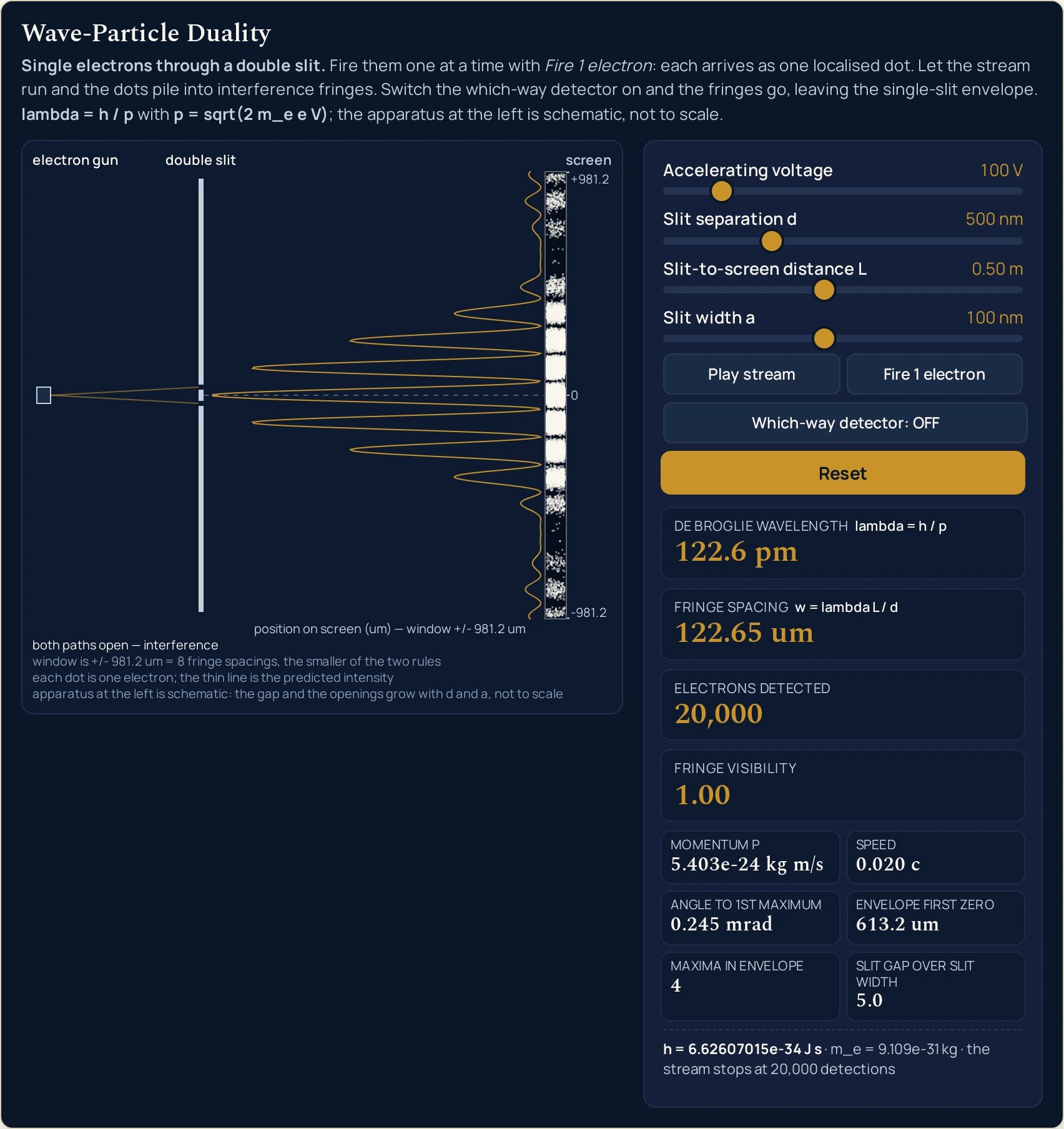
Single electrons through a double slit. Fire them one at a time with Fire 1 electron: each arrives as one localised dot. Let the stream run and the dots pile into interference fringes. Switch the which-way detector on and the fringes go, leaving the single-slit envelope. lambda = h / p with p = sqrt(2 m_e e V); the apparatus at the left is schematic, not to scale.
Load a real case onto the apparatus
Each button writes the four sliders and sets the which-way detector, which together are the whole state, so a load never inherits anything from the last one. It does not clear the screen: the lab keeps the electrons already detected and re-draws them from the new curve, so what you see is the pattern the new setting predicts. Work down the list in order — the first three change one thing at a time, and the fourth changes the question rather than the apparatus.
Pick a case above, or move the four sliders and press the detector yourself.
What Is the Wave-Particle Duality Simulator?
The wave-particle duality simulator is a free interactive physics lab that runs in your browser, with nothing to install and no sign-up. It fires electrons at a barrier with two slits and draws the detection screen one dot at a time, so the two faces of a quantum object arrive separately: each electron is recorded as a single localised hit, and only the pile of hits shows the interference pattern that needed both slits to be open.
Four sliders set the apparatus and one button changes the question being asked. The accelerating voltage runs 20 to 600 V in steps of 20, the slit separation 300 to 1000 nm in steps of 50, the slit-to-screen distance 0.10 to 1.00 m in steps of 0.05, and the slit width 20 to 200 nm in steps of 10. Which-way detector: OFF becomes Which-way detector: ON on one press, and that press is the whole experiment: the fringes vanish and the broad single-slit envelope is all that is left.
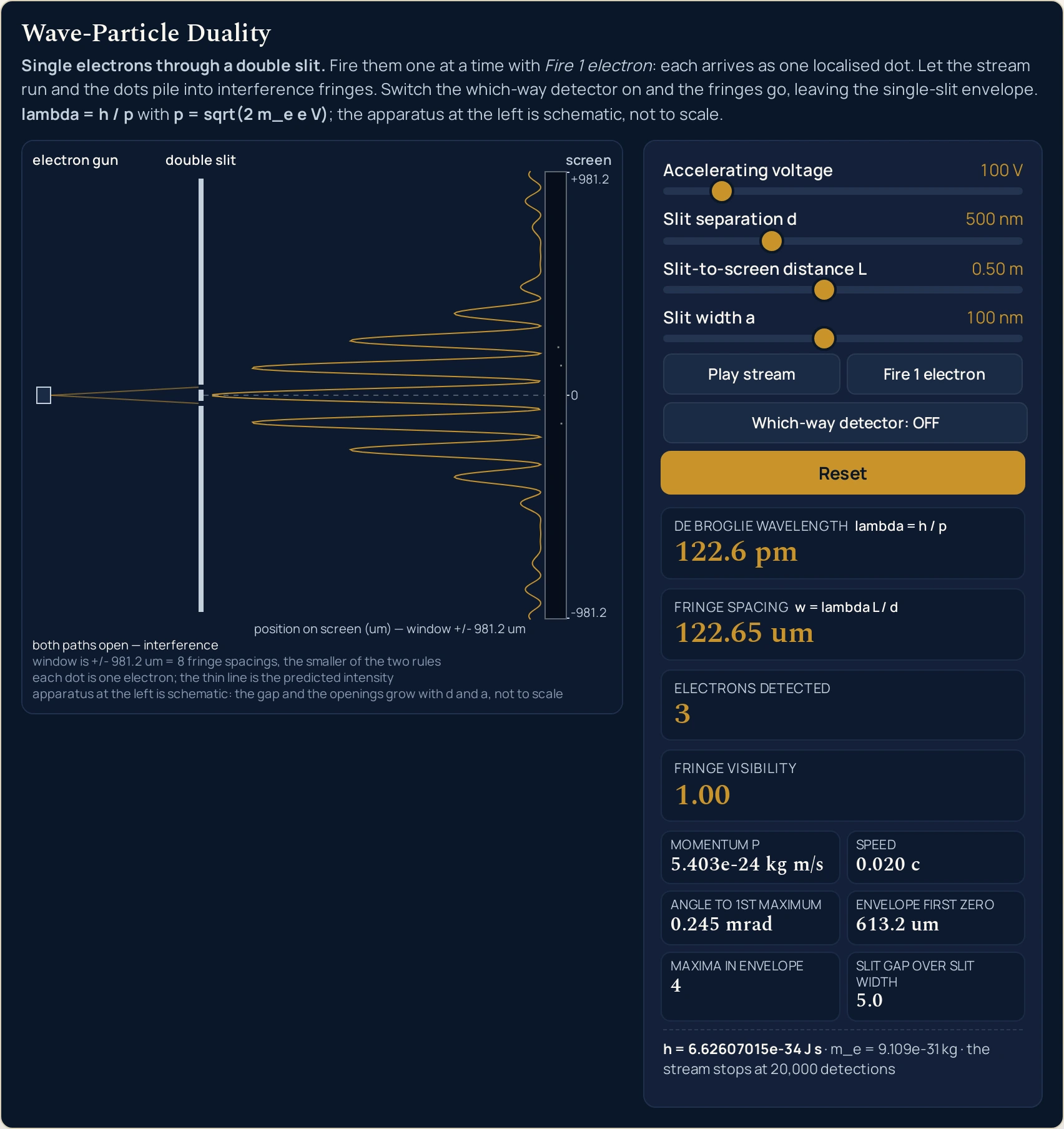
Ten readouts answer. Four cards give the de Broglie wavelength, the fringe spacing, the number of electrons detected and the fringe visibility; six compact cells add the momentum, the speed as a fraction of the speed of light, the angle to the first maximum, the envelope’s first zero, how many maxima fit inside that envelope on one side, and the slit gap divided by the slit width. At the setting the lab boots in they read 122.6 pm, 122.65 um, 1.00, 5.403e-24 kg m/s, 0.020 c, 0.245 mrad, 613.2 um, 4 and 5.0.
The stream starts itself when the page loads and stops itself at 20,000 detections, so the pattern is already building when you arrive. Fire 1 electron pauses the stream and sends exactly one more, which is the state worth looking at: one dot, nowhere near the middle, telling you nothing on its own. Reset clears the dots and the count and leaves the stream paused, so that state is always one click away.
Three things this lab is honest about. The visibility figures 1.00 and 0.00 are the ideal limits of the intensity equation, computed from the model rather than estimated from the dots, and a real which-way measurement decoheres only partly and leaves a visibility between the two. The dot positions come from a seeded pseudo-random generator, which models quantum randomness and is not a quantum random source. The apparatus drawn at the left is schematic: the gap and the openings grow with the slit separation and the slit width, but they are not to scale.
| Control | What it sets | Step or default |
|---|---|---|
| Accelerating voltage | 20 to 600 V | steps of 20 V, boots at 100 V |
| Slit separation d | 300 to 1000 nm | steps of 50 nm, boots at 500 nm |
| Slit width a | 20 to 200 nm | steps of 10 nm, boots at 100 nm |
| Slit-to-screen distance L | 0.10 to 1.00 m | steps of 0.05 m, boots at 0.50 m |
| Which-way detector | OFF or ON | one button, boots OFF |
| Buttons | Play, Fire 1, Reset | the stream boots running |
How to use the wave particle duality simulator
- Do not press anything yet. The stream starts itself when the page loads, so the first button already reads Pause stream and Electrons detected is climbing at roughly 700 a second. The other three cards are at their boot values: De Broglie wavelength 122.6 pm, Fringe spacing 122.65 um and Fringe visibility 1.00.
- Let it finish, or stop it. The stream ends itself at 20,000 detections after about half a minute, at which point Electrons detected reads 20,000 and the button flips to Play stream on its own. Press Pause stream if you would rather freeze it earlier; the picture stays exactly as it was.
- Press Reset, because the empty screen is the point. It clears every dot, takes Electrons detected to 0, stops the stream and leaves all four sliders where you had them. This is the one state the stream can never show you, and it is worth reaching deliberately.
- Press Fire 1 electron three times. Electrons detected reads 1, then 2, then 3, and three marks appear on an otherwise empty strip. Three positions are not a pattern, and that is the honest state of the evidence after three electrons.
- Now press Play stream and watch the same screen fill. The stream runs at roughly 700 detections a second, so the bands appear while you watch, and by the time it stops the marks line up with the peaks of the thin predicted curve and the gaps between them are all but empty. No electron behaved differently from the first three — only the number of them changed.
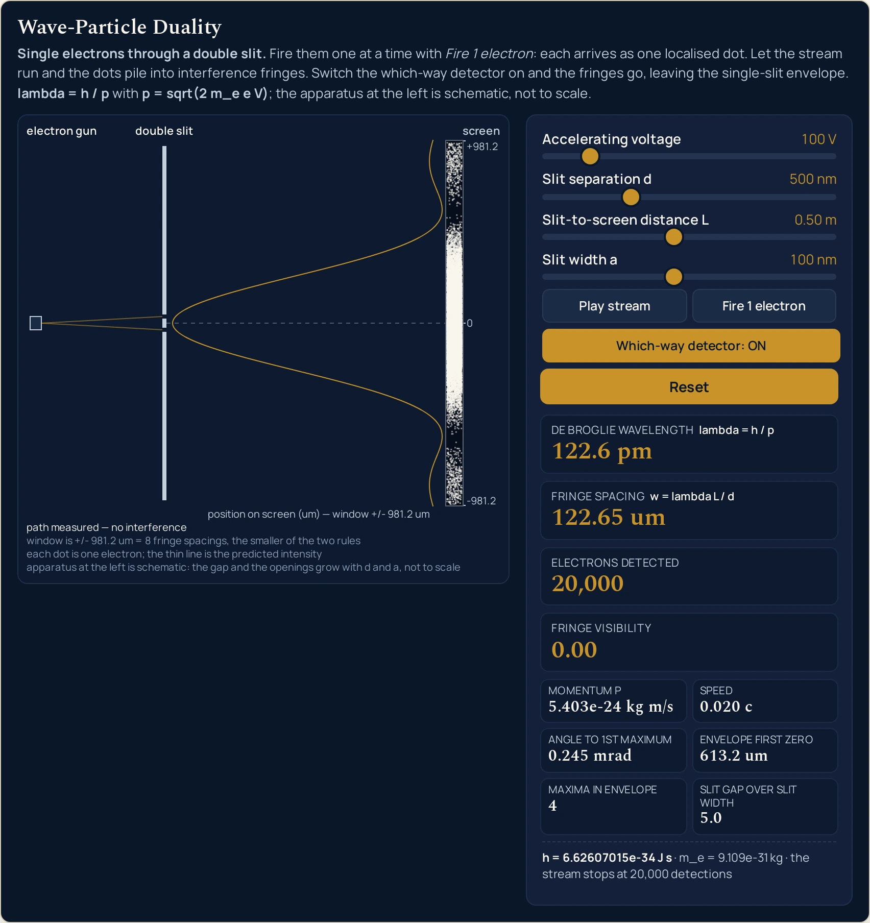
- Press Which-way detector: OFF. The label turns to Which-way detector: ON, Fringe visibility falls from 1.00 to 0.00, and the first caption line under the drawing changes from both paths open — interference to path measured — no interference. Watch the other nine readouts while you do it: not one of them moves.
- Drag the Accelerating voltage slider. It runs 20 to 600 V in steps of 20. De Broglie wavelength and Fringe spacing both move, from 274.2 pm and 274.24 um at the bottom stop to 50.1 pm and 50.07 um at the top, while Maxima in envelope holds at 4 throughout. If you would rather give the electron a mass and a speed than a voltage, that is the job of the de Broglie wavelength calculator.
- Drag Slit width a and keep your eye on the fringe card. It does not move: Fringe spacing stays at 122.65 um from 20 nm all the way to 200 nm. What changes is Envelope first zero, from 3066.2 um down to 306.6 um, and Maxima in envelope with it, from 24 down to 2.
- Read the axis label and the second caption line together. At the boot setting they say
position on screen (um) — window +/- 981.2 umandwindow is +/- 981.2 um = 8 fringe spacings, the smaller of the two rules. The drawing never rescales silently: it states its window in micrometres and names which of its two candidate windows won. - Read the fixed line at the foot of the panel last. It says
h = 6.62607015e-34 J s · m_e = 9.109e-31 kg · the stream stops at 20,000 detections. That is the whole of what the panel assumes, in one line, and it is worth copying alongside any figure you take from here. - One habit worth having: press Fire 1 electron while the stream is running. It stops the stream first and then delivers exactly one more detection, so the count goes up by one and no further. You can therefore step the experiment forward from any point without having to pause it by hand.
The step worth repeating is the sixth one. Load Default double slit, let the fringes build, then press the detector without touching a slider. The stripes fill in and the broad hump of a single slit is left behind, while the wavelength, the momentum, the speed, the angle, the envelope and the fringe spacing all hold their values. What changed was the question the apparatus asks, not the apparatus.
For what duality is — the evidence on both sides, where lambda = h / p comes from, why everyday objects never show fringes, and seven worked problems — read the full guide to wave-particle duality. This page is about the panel and the drawing: what each readout proves, and where the picture gives up before the numbers do.
Worked example: change one thing at a time
Every row below is one setting of the four sliders and the detector, and every cell is a string the running lab printed there. These five settings are the ones this page publishes as presets, so they are also the ones the lab’s own tests pin. Where a cell and the lab ever part company, believe the lab.
| Setting | Wavelength | Fringe spacing | Visibility | Momentum | Envelope first zero | Maxima in envelope |
|---|---|---|---|---|---|---|
| Default double slit | 122.6 pm | 122.65 um | 1.00 | 5.403e-24 kg m/s | 613.2 um | 4 |
| Wider slit gap | 122.6 pm | 61.32 um | 1.00 | 5.403e-24 kg m/s | 613.2 um | 9 |
| Faster electrons | 61.3 pm | 61.32 um | 1.00 | 1.081e-23 kg m/s | 306.6 um | 4 |
| Which-way detector on | 122.6 pm | 122.65 um | 0.00 | 5.403e-24 kg m/s | 613.2 um | 4 |
| Narrow slits, broad envelope | 122.6 pm | 245.29 um | 1.00 | 5.403e-24 kg m/s | 6132.4 um | 24 |
Rows 1 and 2 separate the electron from the apparatus. Doubling the slit separation leaves the wavelength and the momentum untouched — 122.6 pm and 5.403e-24 kg m/s in both — and halves the fringe spacing, 122.65 to 61.32 um. The envelope cell does not move either, because it depends on the slit width and not on the gap. So nine fringes now fit inside the same 613.2 um where four fitted before.
Rows 1 and 3 are the opposite experiment. Four times the voltage halves the wavelength to 61.3 pm, and this time everything about the pattern shrinks with it: the fringe spacing halves to 61.32 um and the envelope halves to 306.6 um, so Maxima in envelope is unchanged at 4. Rows 2 and 3 therefore print the same 61.32 um fringe spacing from two quite different electrons, which is the trap the table is set to catch.
Rows 1 and 4 are the same apparatus asked a different question. Five of the six readings are identical; only Visibility differs, 1.00 against 0.00. Both of those are the ideal limits of the intensity equation and not readings from a detector — the breakdown list below says what a real measurement would leave instead.
The slit width moves the envelope and nothing else
Hold the voltage, the separation and the screen distance at their boot values and walk the Slit width a slider across its whole range. Two columns refuse to move and three change together, and the last of them is the one that decides which order goes missing.
| Setting | Wavelength | Fringe spacing | Envelope first zero | Maxima in envelope | Slit gap over slit width |
|---|---|---|---|---|---|
| Slit width 20 nm | 122.6 pm | 122.65 um | 3066.2 um | 24 | 25.0 |
| Slit width 40 nm | 122.6 pm | 122.65 um | 1533.1 um | 12 | 12.5 |
| Slit width 60 nm | 122.6 pm | 122.65 um | 1022.0 um | 8 | 8.3 |
| Slit width 100 nm | 122.6 pm | 122.65 um | 613.2 um | 4 | 5.0 |
| Slit width 140 nm | 122.6 pm | 122.65 um | 438.0 um | 3 | 3.6 |
| Slit width 200 nm | 122.6 pm | 122.65 um | 306.6 um | 2 | 2.5 |
Read the last two columns against each other. Where the ratio lands on a whole number — 25.0, 12.5 is not one, 5.0 — the count is one less than it, because the order with that number arrives exactly where the envelope has already fallen to zero and is wiped out. Where the ratio is not a whole number, 8.3 or 3.6, nothing is lost and the count is simply the number of whole orders that fit. The spreading of one slit on its own is ordinary diffraction, which the guide to diffraction handles properly.
The 200 nm row is also where the drawing changes its mind about the window. At every other setting in this table the caption reads 8 fringe spacings; at 200 nm it reads window is +/- 919.8 um = 3 envelope first zeros, the smaller of the two rules, because three envelope zeros is now the narrower of the two candidates. The axis label changes with it and the figure is restated in micrometres either way.
Two different electrons, one identical pattern
This is the pair worth dwelling on, and it is a warning rather than a curiosity. Keep the slits 500 nm apart and 100 nm wide, then reach 61.32 um fringes two ways: raise the voltage to 400 V, or leave it at 100 V and bring the screen in to 0.25 m.
| Setting | Wavelength | Momentum | Speed | Angle to first maximum | Fringe spacing | Envelope first zero |
|---|---|---|---|---|---|---|
| 100 V, screen at 0.25 m | 122.6 pm | 5.403e-24 kg m/s | 0.020 c | 0.245 mrad | 61.32 um | 306.6 um |
| 400 V, screen at 0.50 m | 61.3 pm | 1.081e-23 kg m/s | 0.040 c | 0.123 mrad | 61.32 um | 306.6 um |
Both rows draw the same picture. The fringe spacing agrees to the last digit the card prints, the envelope agrees, the maxima count agrees at 4 and the plotted window agrees — yet one electron has twice the wavelength of the other and half its momentum. The cells that separate them are the ones the screen cannot show you on its own: Angle to 1st maximum, 0.245 mrad against 0.123 mrad, and the wavelength, the momentum and the speed behind it.
So a pattern measured in micrometres does not by itself tell you the wavelength. You need the screen distance as well, and that is exactly why a real measurement of a matter wavelength is a measurement of a geometry. The guide to the de Broglie wavelength works the relation through from the other end, and the de Broglie wavelength lab plots it across masses no electron gun could ever reach.
What each control can and cannot move
The table below was compiled from the settings harvested for this page rather than asserted from the formulae: a readout is listed as moving only if it was observed to move across that control’s own range, with the other three held at their boot values. It is the fastest way to find out whether a reading you care about is a property of the electron or of the apparatus.
| Control | What moves | What cannot move |
|---|---|---|
| Accelerating voltage | De Broglie wavelength, Fringe spacing, Momentum, Speed, Angle to 1st maximum, Envelope first zero | Fringe visibility, Maxima in envelope, Slit gap over slit width |
| Slit separation d | Fringe spacing, Angle to 1st maximum, Maxima in envelope, Slit gap over slit width | De Broglie wavelength, Fringe visibility, Momentum, Speed, Envelope first zero |
| Slit-to-screen distance L | Fringe spacing, Envelope first zero | De Broglie wavelength, Fringe visibility, Momentum, Speed, Angle to 1st maximum, Maxima in envelope, Slit gap over slit width |
| Slit width a | Envelope first zero, Maxima in envelope, Slit gap over slit width | De Broglie wavelength, Fringe spacing, Fringe visibility, Momentum, Speed, Angle to 1st maximum |
| Which-way detector | Fringe visibility, the drawn curve, the first caption line | all nine other readouts |
Three patterns fall out of it. Only the voltage touches the electron itself, so only the voltage can move the wavelength, the momentum and the speed. The screen distance is pure magnification: it moves the two lengths measured on the screen and nothing else, not even the angle. And the detector button moves exactly one number, which is what makes it an argument rather than a knob.
Formula and symbol reference
The panel prints its two relations on itself, inside the labels of the cards they feed. lambda = h / p sits above the De Broglie wavelength card and w = lambda L / d above the Fringe spacing card, so neither answer arrives without the rule that produced it. Neither is derived here.
Behind the first of them is a third relation, printed in the lab’s opening band but on none of the cards: the momentum an electron picks up falling through a potential difference, p = sqrt(2 m_e e V), which is where the voltage slider gets in. Where that relation comes from, and the arithmetic of turning a mass and a speed into a wavelength, belongs to the de Broglie wavelength guide rather than to this panel.
| Symbol | Meaning | SI unit | In this lab |
|---|---|---|---|
| V | Potential difference the electron is accelerated through from rest. It is the only control that changes what the electron is rather than where the apparatus sits | volt | 20 to 600 in steps of 20, printed beside the slider: “20 V”, “100 V” (the boot value), “600 V”. |
| d | Separation of the two slits, centre to centre. It sets how finely the two paths interfere, and with the slit width it fixes which order goes missing | metre (the slider is in nanometres) | 300 to 1000 in steps of 50: “300 nm”, “500 nm” (the boot value), “1000 nm”. |
| L | Distance from the barrier to the detection screen. It magnifies the pattern without touching the physics upstream of it | metre | 0.10 to 1.00 in steps of 0.05: “0.10 m”, “0.50 m” (the boot value), “1.00 m”. |
| a | Width of each slit. It sets the single-slit envelope the fringes have to live inside, and nothing else | metre (the slider is in nanometres) | 20 to 200 in steps of 10: “20 nm”, “100 nm” (the boot value), “200 nm”. Always smaller than d, by construction of the two ranges. |
| p | Momentum the electron leaves the gun with, in the Momentum p cell. The card above it prints the relation that produced it | kilogram metre per second | a three-decimal mantissa: “2.416e-24 kg m/s” at 20 V, “5.403e-24 kg m/s” at the boot setting, “1.323e-23 kg m/s” at 600 V. |
| lambda | De Broglie wavelength of that electron, on the headline card. Its own label prints lambda = h / p, so the answer never arrives without the rule |
metre (the card is in picometres) | one decimal of a picometre: “274.2 pm” at 20 V down to “50.1 pm” at 600 V, with “122.6 pm” at the boot setting. |
| w | Spacing between neighbouring bright fringes on the screen, on the second card, whose label prints w = lambda L / d |
metre (the card is in micrometres) | two decimals of a micrometre: “24.53 um” at the near screen stop, “122.65 um” at the boot setting, “274.24 um” at 20 V. |
| theta | Angle from the axis to the first bright fringe, in the Angle to 1st maximum cell. It is what the fringe spacing looks like before the screen distance magnifies it | radian (the cell is in milliradians) | three decimals of a milliradian, and small everywhere: “0.050 mrad” at the shortest wavelength and widest gap, “0.245 mrad” at the boot setting, “0.914 mrad” at the longest wavelength and narrowest gap, which is 20 V with d at 300 nm. Only V and d move this cell at all. |
| envelope first zero | Where one slit on its own sends nothing, from a sin(theta) = lambda. In the Envelope first zero cell, measured on the screen like the fringe spacing |
metre (the cell is in micrometres) | one decimal of a micrometre: “306.6 um” at the widest slits, “613.2 um” at the boot setting, “3066.2 um” at the narrowest. |
| visibility | Contrast of the fringes, on the fourth card. It is computed from the intensity equation’s limits, not estimated from the dots on the screen | none (a ratio) | two decimals, and only ever two values: 1.00 with both paths open and 0.00 once the detector is on. |
| h | The Planck constant, in the fixed line under the readouts. Exact by the 2019 definitions of the SI units | joule second | a constant: 6.62607015e-34 J s, the value the reused De Broglie calculator already uses, so the two pages of this cluster cannot disagree. |
| m_e | Electron mass, also in the fixed line. Pinned to the live calculator’s own default rather than to the CODATA figure, which would differ in the fourth digit | kilogram | a constant: 9.109e-31 kg. |
The row worth reading twice is the visibility. It is the only readout on the panel that is not a number computed from a setting but a limit of the equation being plotted, and it is also the only one with just two possible values. Everything else on the panel is continuous in the sliders that drive it.
The physics: what the dots and the fringes each tell you
Everything to the right of the barrier is placed by one vertical map. A position on the screen in micrometres becomes a height in pixels, and both the marks and the predicted curve go through that same map. That is the single decision that makes the drawing arguable rather than decorative: the dots filling the curve is a claim, not a coincidence of two separately drawn pictures.
So the two halves of the drawing answer two different questions. One mark is a measurement — this electron, this position, whole and localised — and it carries no information about the stripes at all. The curve is a statement about probability, and it needs a sample before anything can be checked against it.
That is why the three-dot state matters more than the finished pattern. After three detections nothing on the screen distinguishes the two-slit prediction from the one-slit one. After twenty thousand, the bands and the empty gaps between them are the most obvious thing on the canvas, and no individual electron did anything different on the way.
The window the drawing plots is chosen, not fixed, and the caption says which rule chose it. Three envelope first zeros and eight fringe spacings are both reasonable framings, and the lab takes the narrower of the two so that the pattern always fills the strip. Because both figures move with the sliders, the rule that wins can change under you — which is why the figure is restated in micrometres on the axis every time.
The envelope deserves its own sentence, because it is the half of the picture that is not about interference. Each slit on its own spreads the beam, and that spreading sets a ceiling the fringes have to live under; the Envelope first zero cell is where that ceiling first touches zero. Fringes do not fade because the electrons get tired — they fade because the single-slit factor is falling.
The which-way result is the one the whole apparatus exists for, and the panel states it in the plainest way it can. One press, one number: 1.00 to 0.00. Nothing is dimmed and nothing is narrowed, and the envelope cell proves it by not moving — what the measurement removes is the modulation inside the envelope, not the envelope.
There is a reason that trade is so unforgiving rather than merely awkward. One press of the button does what tying each electron to an opening would do: it throws away the sideways momentum that put the fringes where they were, and the fringes have nothing left to stand on. The guide to the Heisenberg uncertainty principle sets that exchange out away from any particular apparatus, and the uncertainty principle lab lets you push on it directly.
Narrow the browser and the drawing gives things up in a fixed order rather than shrinking everything. The caption lines shorten first, then stop from the bottom upwards, so the mode line is the last thing to go and a strip that cannot hold it holds nothing at all. The window figure survives in the axis label in every form that is drawn at all, so the scale is never left unstated.
Where the wave-particle duality simulator breaks down
The lab solves its own model exactly, so nothing on the screen ever fails. Everything below is a limit of that model, of the slider grid, or of what a drawing a few hundred pixels wide can carry, and each item says what this lab does about it.
- The two visibility values are the equation’s limits, not a detector’s output
- The card prints 1.00 with both paths open and 0.00 once the path is measured, and both are computed from the intensity relation the lab plots rather than estimated from the dots. Real hardware is neither a perfect detector nor a perfectly gentle one: it degrades the coherence only in part, so the contrast it leaves sits between the two, and pinning that number down for a given instrument is a measurement rather than an application of this panel. No measured visibility, decoherence time or coherence length appears anywhere here, because none was sourced for this cluster.
- The randomness is a seeded generator, not a quantum source
- Every mark the stream lays down is placed by a fixed-seed generator, tuned so that the histogram of marks converges on the curve drawn beside them. That reproduces quantum randomness in distribution only; no browser can draw on a quantum source. Because the seed never changes, the same sequence of clicks rebuilds the same picture — useful for teaching, and the opposite of what a real experiment does.
- The apparatus at the left is schematic, and says so
- The gap between the openings grows when you raise the slit separation and each opening grows when you raise the slit width, so the drawing is not static — but it is not to scale, and the fourth caption line states that on the canvas itself. The real proportions are hopeless to draw: slits hundreds of nanometres apart, a screen half a metre away. Only the vertical axis to the right of the barrier is a real scale, and it is the one the readouts are quoted against.
- Non-relativistic only, which is why the speed cell is on the panel
- Across every setting the four sliders can reach, the speed cell runs from 0.009 c to 0.048 c, so the Lorentz factor exceeds 1 by 1.18e-3 at worst and the relativistic correction to the wavelength is about 0.03 per cent — below the one tenth of a picometre the card displays. The panel shows the speed rather than asking you to take that on trust. Push an electron gun past this range in real life and the relation the card prints is no longer the one to use.
- The small-angle fringe formula is safe here and not in general
- The Angle to 1st maximum cell never exceeds 0.914 mrad anywhere the four sliders can reach together, which holds the gap between the evenly spaced form the fringe card uses and the exact geometry under one part in a million. At larger angles it does not, and the fringes stop being evenly spaced at all. Do not carry the card’s formula into an apparatus with wider angles than this one has.
- Do not re-derive one readout from another
- Every figure is computed from the exact value and rounded once, so a chain of rounded figures need not close. Take the printed 122.6 pm, multiply by the 0.50 m screen distance and divide by the 500 nm separation, and you get 122.6 um — while the card beside it prints 122.65 um, because it used the unrounded wavelength. Read each figure from the cell that publishes it.
- The envelope always has a first zero on this axis
- The Envelope first zero cell is a real position on the screen at every setting the sliders can reach, because the wavelength is at most about one seventieth of the slit width anywhere in the box — the ratio never exceeds 0.0137. A wavelength longer than the slit would have no first zero to report, and that case is simply not reachable here, so nothing in the drawing or the panel describes it.
- The screen is only as wide as the stated window
- The plotted window is also the range the marks are drawn from, so no electron is ever placed outside it. That keeps the picture and the curve honest about each other, and it means the counts are not a model of a real detector’s acceptance: a real screen catches whatever arrives, including whatever would have fallen outside the plotted window.
- Plenty is left out of the apparatus
- Nothing outside the four sliders and the one button exists in this model: electrons never push on one another on the way across, every arrival is counted, nothing clips the edge of an opening, and no stray field or bench vibration ever nudges a mark. There is no electron optics either. A real instrument puts magnifying optics between the barrier and its detector, because the fringe spacing here runs from 5.01 um to 914.14 um across its slider range, under a millimetre even at its coarsest; the strip in this panel magnifies nothing. Nothing on this page describes a real instrument, and no voltage, slit width, date, laboratory or experimenter is attached to any claim.
- This lab says nothing about light
- Duality runs in both directions, and only the matter half is modelled here. That light hands over its energy in indivisible packets is the other half of the evidence, and it belongs to the guide to the photoelectric effect and its own lab. There is no work function, no threshold and no photon anywhere in this panel.
- The stream is finite, and the count is not a rate
- The stream delivers roughly 700 detections a second of wall clock and stops itself at 20,000, after which Play stream will not restart it until you press Reset. Those figures are properties of the animation, not of any beam: a real source would be quoted as a current, and nothing on this panel is one.
- Nothing here has been measured
- Four slider positions and one button state go in, and one idealised pattern comes out. A preset name is only a label for the five values it writes. Check anything you intend to depend on against a source of your own first.
Where wave-particle duality is actually used
- Picking an accelerating voltage for a wavelength you need
- This is the question the voltage slider answers directly. The card runs from 274.2 pm at the 20 V stop down to 50.1 pm at 600 V, which brackets the few hundred picometres that neighbouring atoms in a solid sit apart — the reason an electron beam diffracts usefully from a crystal at all. Treat the figures as an order of magnitude and verify the spacing you actually care about before use.
- Working out whether a pattern would be measurable before building anything
- Read the fringe card against whatever detector you have. At the default separation it runs from 24.53 um with the screen at 0.10 m to 245.29 um at 1.00 m, so moving the screen is the cheapest magnification available. That is also the honest reason real instruments add electron optics rather than relying on the screen distance alone.
- Settling the “the electrons are bumping into each other” objection in front of a class
- Press Reset, then Fire 1 electron three times, and let someone describe what they see: three marks, no stripes, Electrons detected 3. Then press Play stream and let the same screen fill. Nothing in the apparatus changed between the two states, which removes the objection without anyone having to argue it.
- Showing that a measurement is not a disturbance you could make gentler
- Put the detector on and off while the audience watches the Fringe visibility card and the nine readouts beside it. 1.00 to 0.00, and nothing else moves at all. The usual follow-up — could a more delicate detector leave some fringes? — is a real question, and the honest answer is the one in the breakdown list: a partial measurement leaves a partial visibility, which this idealised model does not reach.
- Reading a missing order straight off the panel
- Compare the Slit gap over slit width cell with Maxima in envelope. At the boot setting they read 5.0 and 4: order five lands exactly on the envelope zero and is lost. Set the slit width to 40 nm for 12.5 and 12, where the ratio is not a whole number and nothing goes missing. One glance at two cells answers a question that otherwise needs two equations solved against each other.
- Auditing a wavelength and a momentum someone has handed you
- Multiply the Momentum p cell by the De Broglie wavelength card and you should get the Planck constant back. At the boot setting that is 5.403e-24 times 122.6 pm, or 6.624e-34, against the 6.62607015e-34 the fixed line prints — agreement in the third digit, which is as much as two rounded cards can give. A factor-of-ten slip shows up instantly; a fourth-digit disagreement is just the rounding.
- Teaching the difference between a property of the object and a property of the rig
- The control table above is the lesson in one page. The wavelength, the momentum and the speed belong to the electron and only the voltage can touch them; the fringe spacing and the envelope belong to the geometry and three different sliders move them. Students who can sort a panel into those two groups rarely misread a formula afterwards.
- Showing that the same pattern does not mean the same particle
- Load Faster electrons, note the 61.32 um fringes, then go back to 100 V and bring the screen in to 0.25 m. The fringe card, the envelope cell and the maxima count all return to the same values from a wavelength twice as long. It is the cleanest available argument that a measured spacing is not a measured wavelength until the geometry is known. For the photon side of the same relation, the photon energy calculator starts from a wavelength instead of a voltage.
Where to go next
The topic itself — what wave-particle duality is, the evidence on both sides, where lambda = h / p comes from, what happens when you ask which slit, why everyday objects show no fringes, and seven problems worked end to end — is in Wave-Particle Duality: One Electron, Two Slits. If you would rather type a mass and a speed than drag a voltage, the de Broglie wavelength calculator runs the same relation in three directions.
The neighbouring questions have tools of their own. The de Broglie wavelength guide and its lab own the relation itself; the photoelectric effect guide with its lab and its calculator cover the half of duality that is about light; and the guide to diffraction alongside the diffraction lab covers the single-slit spreading that sets the envelope here.
Further out, the guide to the Heisenberg uncertainty principle is where the which-way trade is handled properly, the quantum mechanics overview places duality among the ideas it belongs with, and the photon energy formula guide with its calculator handles a photon rather than an electron. The rest is in the library of physics simulations and on the blog.
Frequently asked questions
Dots were already piling up before I touched anything. Did I miss the start?
No — the stream starts itself when the page loads, so the Play button reads Pause stream and Electrons detected is already climbing. Nothing was missed, but the state worth seeing is the empty one. Press Reset: the dots and the count go to zero, the stream stops, and the button flips to Play stream. Now Fire 1 electron three times and watch Electrons detected read 1, then 2, then 3.
Why does Reset leave the stream paused instead of starting it again?
Because the whole argument of the lab is unreachable otherwise. At roughly 700 detections a second, several hundred dots land before anyone can reach Fire 1 electron, so a Reset that resumed the stream would make a screen with three dots on it impossible to see. Reset therefore clears the dots and the count, stops the stream and leaves all four sliders exactly where you had them.
I switched the which-way detector on and only one number changed. Is that right?
Yes, and it is the cleanest single result in the lab. Fringe visibility falls from 1.00 to 0.00 and the first caption line changes from both paths open to path measured, while the other nine readouts hold: the wavelength, the fringe spacing, the momentum, the speed, the angle, the envelope zero, the maxima count and the slit ratio are all unchanged. Measuring the path removes the stripes, not the electrons.
Is the fringe visibility measured from the dots on the screen?
No. It is computed from the intensity equation the lab plots, and the two values it can print, 1.00 and 0.00, are that equation’s ideal limits. An estimate taken from the dots would wobble with every frame while the physics stood still, because early on there are only a handful of them. A real which-way measurement decoheres only partly and would sit somewhere between the two.
Why does the slit width change the envelope but leave the fringe spacing alone?
Because the two come from different lengths. Fringe spacing is the wavelength times the screen distance divided by the slit separation, and the slit width is not in it. The width sets how far one opening spreads the beam on its own, which is the envelope. Drag Slit width a from 100 nm to 20 nm and Fringe spacing holds at 122.65 um while Envelope first zero goes from 613.2 um to 3066.2 um.
Why does the fringe spacing card not match what I get from the other two cards?
Because each card is computed from the exact value and rounded once. Take the printed 122.6 pm, multiply by 0.50 m and divide by 500 nm, and you get 122.6 um, whereas the card prints 122.65 um — it used the unrounded 122.6452 pm. Read each figure from the cell that publishes it rather than rebuilding it from a neighbour.
What does "the smaller of the two rules" in the caption mean?
The drawing has to choose how much of the screen to plot, and it takes whichever of two candidate windows is narrower: three envelope first zeros, or eight fringe spacings. At the setting the lab boots in, eight fringe spacings wins and the caption reads window is +/- 981.2 um = 8 fringe spacings, the smaller of the two rules. Widen the slits to 200 nm and the other rule takes over.
Is the randomness in the dot positions real quantum randomness?
No, and no browser could supply it. A fixed-seed generator places each mark, with the odds set so that the pile of marks settles onto the intensity curve the lab draws beside it. That is quantum randomness reproduced in distribution, not sampled from a quantum source. Because the seed never changes, the same sequence of clicks gives the same picture twice.
References & formula source
- Two relations drive the whole panel. The de Broglie card applies lambda = h / p, with the momentum of an electron accelerated from rest through a potential difference V taken as p = sqrt(2 m_e e V); the fringe card applies w = lambda L / d. The fixed line under the readouts prints the two constants they use, h = 6.62607015e-34 J s and m_e = 9.109e-31 kg, and neither is derived on this page.
- The constants are pinned to the live De Broglie wavelength calculator this cluster reuses rather than to CODATA, deliberately. The Planck constant and the elementary charge, 1.602176634e-19 C, are exact by the 2019 definitions of the SI units. The electron mass is the calculator's own default, 9.109e-31 kg; substituting the CODATA figure would make the lab and the calculator disagree in the fourth digit of every wavelength they both print.
- The two visibility values this lab can print, 1.00 and 0.00, are the ideal limits of the intensity equation it plots, computed from the model and not estimated from the dots. A real which-way measurement is neither perfect nor perfectly gentle: it spoils the coherence only in part, and a working apparatus would land between those two numbers rather than on either. Nothing in this simulation describes a specific apparatus, and no measured visibility, decoherence time or coherence length is quoted anywhere, because none was sourced for this cluster.
- The electrons are treated non-relativistically, and that is justified rather than assumed. Across the slider range the speed cell runs from 0.009 c at 20 V to 0.048 c at 600 V, which the panel shows rather than asking you to take on trust; the Lorentz factor exceeds 1 by 1.18e-3 at the top of that range and the relativistic correction to the wavelength is about 0.03 per cent, below the one tenth of a picometre the card displays.
- The small-angle form of the fringe spacing is exact to the precision shown here and is not a general licence. The angle cell never exceeds 0.914 mrad anywhere the four sliders can reach together, which holds the gap between w = lambda L / d and the exact L tan(theta) under one part in a million. At larger angles they do not, and the fringes stop being evenly spaced.
- Marks are placed by a fixed-seed generator, so the lab reproduces quantum randomness in distribution only and is not a quantum random source. The apparatus drawn at the left is schematic: the gap between the openings grows with the slit separation and each opening grows with the slit width, but neither is to scale, and the caption says so on the drawing itself. The screen plotted is only as wide as the stated window, which is also the range the dots are drawn from.
- Every readout figure quoted above is a string this simulation printed for the four slider positions and the detector state named beside it, read back out of the running lab rather than worked out by hand. Each is computed from the exact value and rounded once, so re-deriving one printed figure from another will not always reproduce it. Where a figure here and the lab ever part company, believe the lab, and verify anything you intend to rely on against your own data before you quote it.
- No real experiment is described anywhere on this page. There is no apparatus, voltage, slit width, date, laboratory or experimenter attached to any claim, because no source for one was fetched for this cluster. A working interferometer would also sit behind magnifying optics, since the fringe spacing this panel prints is a few micrometres at its finest and still under a millimetre at its coarsest; none of that optics is modelled here.
- Further reading: Wave–particle duality — Wikipedia