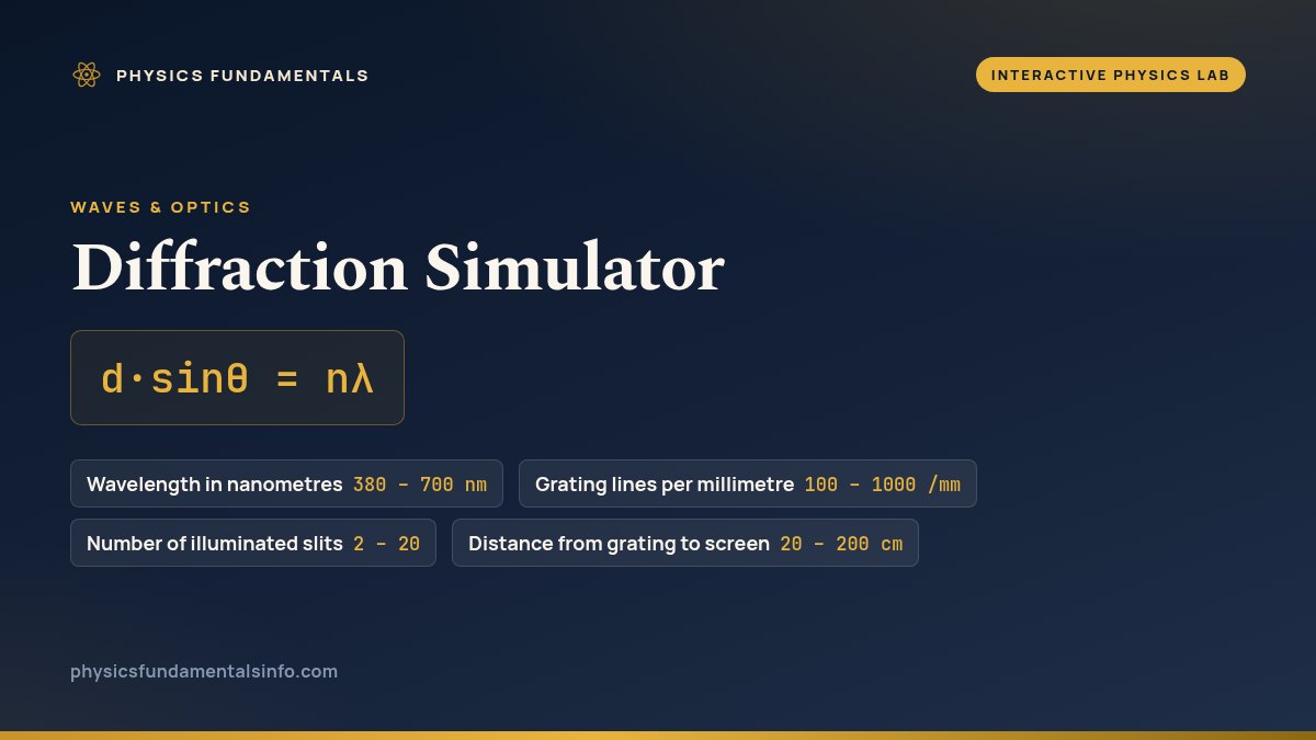
Diffraction through a grating sends bright fringes only where waves from every slit arrive in step — d·sinθ = nλ. Drag the sliders below to change the wavelength, line density, slit count and screen distance, and watch the ray fan and the on-screen intensity pattern respond live.
Diffraction Grating
Monochromatic light hits a grating and fans into ordered bright fringes at d sin(angle) = n·(wavelength). Drag the sliders to move the orders, sharpen them with more slits, and spread them on the screen.
What Is the Diffraction Simulator?
The diffraction simulator is a free interactive physics lab that runs in your browser — nothing to install and no sign-up. Drag the wavelength, line density and slit count to watch the bright orders move and see d sin θ = nλ in action. It reports First-order angle d sin as you drag the sliders.
| Control | Range | Step |
|---|---|---|
| Wavelength in nanometres | 380 – 700 nm | 5 |
| Grating lines per millimetre | 100 – 1000 /mm | 10 |
| Number of illuminated slits | 2 – 20 | 1 |
| Distance from grating to screen | 20 – 200 cm | 5 |
What Each Slider Proves About the Grating Equation
The wavelength slider is the equation working in plain sight: since d·sinθ = nλ pins each bright order to its angle, dragging toward red pushes every order outward and dragging toward violet pulls the whole fan back in. The colour of the rays and the intensity trace follows the slider, so you can literally watch a longer wavelength demand a bigger angle.
The line density slider changes d itself: more lines per millimetre means a smaller slit spacing, and the readout updates d = 1/N as you drag. The orders spread wider apart — and, at the same time, fewer of them survive, because an order only exists while nλ/d ≤ 1. The readouts show the trade live: the first-order angle climbs while the highest visible order falls. You can confirm nmax = floor(d/λ) yourself against the fringe count, or hand the same numbers to the diffraction grating calculator for the full worked steps.
The number of slits is the subtle one, and it corrects the classic misconception directly: this sim's bright fringes are the maxima of the grating equation, not the single-slit minima, and adding slits does not move them at all. What changes is their sharpness — the bottom panel's peaks grow taller and needle-thin as N rises, because more slits cancel the light more completely between the maxima. That sharpening is the whole reason real gratings carry thousands of lines.
Finally, the screen distance turns angles into positions: each fringe lands at y = D·tanθ, so doubling D doubles the spacing on the screen without touching a single angle. It is the same geometry a spectrometer uses to convert an angle measurement into a wavelength — light whose speed in vacuum is the fixed speed of light, whatever its colour.
Where the ideal diffraction grating breaks down
The intensity trace in the lower panel comes from a formula that treats every slit as infinitely narrow, which is why all its peaks stand at the same height. A real grating's slits have a width a, and the whole pattern gets multiplied by a single-slit envelope, (sinα/α)² with α = πa·sinθ/λ, so orders far from the centre arrive visibly dimmer. Worse, wherever d/a is a whole number the envelope's zero lands exactly on an order and erases it — rule the slits half the period wide and every even order simply vanishes.
One wavelength at a time is the second idealisation. Feed a real grating white light and each order becomes a spread-out spectrum, and those spectra eventually collide. What fixes an order is the path difference nλ, so third-order violet is worth 3 × 380 = 1140 nm while second-order red is worth 2 × 700 = 1400 nm: the violet falls inside the red band. From the third order onward the visible spectra sit on top of one another, which is why spectrometers put an order-sorting filter before the detector.
Notice, too, what d·sinθ = nλ never tells you: how much light reaches each order. It settles the angles and nothing else. A plain grating throws most of the incoming energy straight into the useless zeroth order, where every wavelength overlaps. Real instruments cut the grooves as a sawtooth, tilting each facet so the light it reflects specularly lands in a chosen order — a blazed grating can put well over half its light into first order near its design wavelength. The equal peaks here are a geometry answer, not an energy one.
Finally, y = D·tanθ assumes a plane wave reaches the grating and a flat screen catches the result. Neither comes free. An uncollimated source sends rays in over a spread of angles, and each draws its own slightly shifted copy of the pattern, smearing every fringe — which is why a real bench puts a collimating lens ahead of the grating. And because the screen is flat, position grows as tanθ rather than θ: at the default 100 cm the first order lands at 28.6 cm, but pull the screen in to 20 cm and it sits at just 5.7 cm.
Where this is actually used
The rainbow sliding across a CD under a lamp is this equation at work. The data spiral has a track pitch of 1.6 µm, so the disc is a reflection grating of 625 lines per millimetre — inside this lab's own range. Set Line density to 630 /mm and the readout gives d = 1.59 µm; put the wavelength at 650 nm, a red laser pointer, and the first order leaves at 24.17°. A DVD packs its tracks at 0.74 µm, about 1,350 lines/mm, which is exactly why a DVD fans the same lamp into a wider rainbow than a CD does.
A bench spectrometer uses the grating to measure wavelength, and its ceiling is the resolving power R = nN — the order times the number of slits the beam actually covers. Sodium's two yellow lines lie at 589.0 nm and 589.6 nm, so separating them needs R ≈ 980. This lab's slit slider stops at N = 20, giving R = 20 in first order: a resolution of 550/20 = 27.5 nm, which would smear the entire yellow region into one blob. Widen a real beam to 25 mm across a 600 lines/mm grating and it illuminates 15,000 slits, so R = 15,000 and the resolution is 0.04 nm — the doublet splits cleanly. Set the sim to 600 /mm at 590 nm and it puts that first order at 20.73°.
The same counting decides what you can probe at all. An order exists only while nλ/d ≤ 1, so nmax = floor(d/λ): push Line density to its 1,000 /mm maximum with 700 nm light and d = 1.00 µm leaves nmax = 1, just three fringes on the screen. Atomic planes in table salt sit 0.282 nm apart, and against 550 nm light d/λ is 0.0005, so no order exists at all — visible light can never image a crystal lattice. Swap in copper X-rays at 0.154 nm and the first reflection appears near 15.9°, by the same argument at a thousandth of the wavelength (Bragg's version carries an extra factor of two, because the beam reflects from successive planes).
Frequently asked questions
How do I use this diffraction simulator?
Drag the four sliders and watch both panels respond: the wavelength slider moves every bright order, the line-density slider sets the slit spacing d, the slit-count slider sharpens the fringes, and the screen-distance slider spreads them across the screen. The readouts always show d, the first-order angle, the highest visible order and the total fringe count.
Why do the bright spots spread out when I increase the wavelength?
Because the grating equation d sin(angle) = n(wavelength) fixes each order's angle, and a longer wavelength needs a larger sine to keep the equation balanced. Slide from violet 380 nm toward red 700 nm and every order marches outward — the same reason a grating fans white light into a spectrum with red bent furthest.
What does adding more slits change?
Only the sharpness. The bright maxima sit wherever d sin(angle) = n(wavelength), which does not involve the slit count — but with more slits the waves cancel more completely everywhere else, so each fringe becomes taller and narrower. That is exactly why real gratings rule thousands of lines: needle-sharp fringes make precise wavelength measurements possible.
Does this show single-slit or grating diffraction?
Grating (multi-slit) diffraction. The bright peaks here are the maxima of d sin(angle) = n(wavelength). A single slit obeys the similar-looking a sin(angle) = m(wavelength), but that formula locates the dark minima of its pattern, not bright fringes — mixing the two is the classic diffraction mistake.
How many bright orders should I see?
Count n_max = floor(d/wavelength) on each side of the central maximum, giving 2·n_max + 1 fringes in total. With 500 lines/mm (d = 2.00 micrometres) and 550 nm light, d/wavelength = 3.6, so three orders fit each side — seven bright fringes. Raise the line density and watch the count fall as the pattern spreads.
References & formula source
- E. Hecht — Optics, chapter on Fraunhofer diffraction and the diffraction grating.
- Young & Freedman — University Physics with Modern Physics, chapter on Diffraction.
- R. Nave — HyperPhysics, Georgia State University, "Diffraction Grating" section.
- Further reading: Diffraction grating — Wikipedia