The electric potential lab simulator is a free interactive lab built around one piece of arithmetic: V = k·Q1 / r1 + k·Q2 / r2, two signed numbers added together and nothing else. Two point charges sit on a line, a probe slides along that line, and ten readouts answer at once. The two that matter are the Total potential at the probe card and the Net field along x card, because the whole lab exists to show you that they reach zero in different places — and that flipping one charge’s sign makes them swap.
Electric Potential
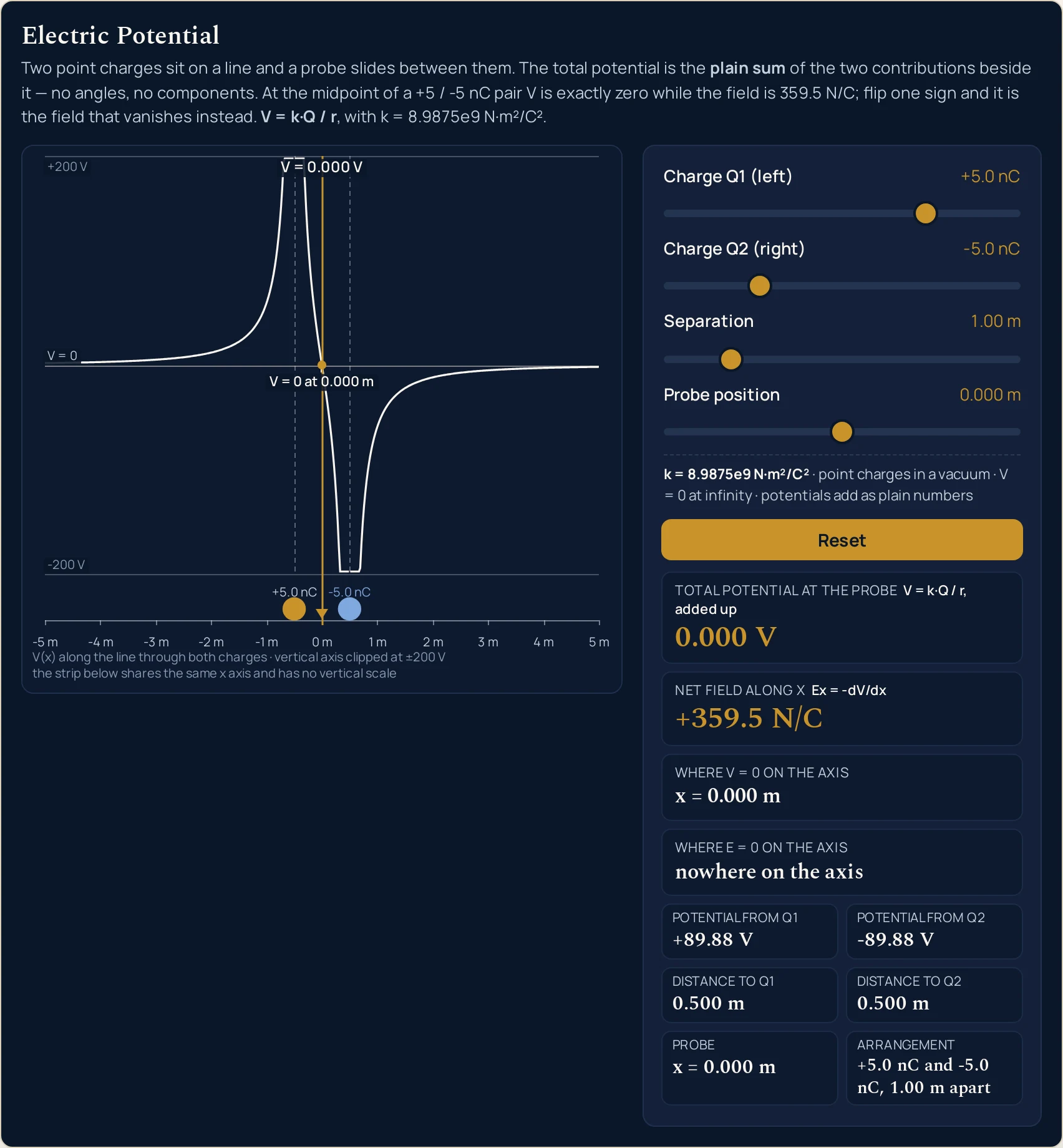
Two point charges sit on a line and a probe slides between them. The total potential is the plain sum of the two contributions beside it — no angles, no components. At the midpoint of a +5 / -5 nC pair V is exactly zero while the field is 359.5 N/C; flip one sign and it is the field that vanishes instead. V = k·Q / r, with k = 8.9875e9 N·m²/C².
Load a real arrangement onto the axis
Each button writes the lab’s own four sliders — both charges, the separation and the probe — and then lets its own update run. Those four values are the entire state, so a load never inherits anything from the one before it. Take them in order: the first two are the same two charges with a single sign flipped, and the last three pull the special places apart until they are plainly three different points.
Pick an arrangement above, or move the four sliders yourself.
What Is the Electric Potential Lab Simulator?
The electric potential lab simulator is a free interactive physics lab that runs in your browser, with nothing to install and no sign-up. Two point charges sit on a line, a probe slides along it, and the panel reports the potential at the probe as a single signed number. That number is the plain sum of the two contributions printed beside it, which is the whole reason potential is worth having: no angles, no components, just arithmetic.
One shared horizontal scale carries the whole drawing, fixed at -5 to +5 m so that nothing rescales as you drag and every screenshot is comparable. The upper region plots V against x with a labelled zero line and a dashed asymptote at each charge, and the vertical axis is clipped rather than allowed to run away. The caption prints the clip it used, for example vertical axis clipped at ±200 V, instead of truncating quietly. The strip underneath shares that same x axis, draws the charges as filled circles sized by magnitude and coloured by sign, and has no vertical scale of its own, which the caption also states.
Four sliders and one button are the entire control set: each charge over -10 to +10 nC in steps of 0.1, the separation over 0.4 to 4 m in steps of 0.05, the probe over -5 to +5 m in steps of 0.005, and Reset. Ten readouts answer. Four cards give the total potential, the net field along x, where V is zero on the axis and where the field is zero; six compact cells add each charge’s own contribution, the distance to each charge, the probe position and the arrangement written out in words.
The two cards that name places ignore the probe completely. Drag the probe the whole length of the axis and x = 0.400 m and 0.625 m does not move, because where the potential vanishes is a property of the two charges and their spacing, not of where you happen to be standing. Flip one charge’s sign and the two cards trade places: a +5.0 nC and -5.0 nC pair reads 0.000 V at its midpoint with a field of +359.5 N/C, and the same pair made alike reads +179.8 V there with a field of 0.000 N/C.
Two limits are printed on the page rather than left implied. The zeros this lab finds are the zeros on that line: the set where V is zero is really a surface, and only where it cuts the axis is drawn. And the zero of potential is a convention, taken infinitely far away here, so a negative reading is a statement about that choice and not about a shortage of anything. A probe placed exactly on a charge prints an em dash in six readouts instead of a number, because the potential of an idealised point charge is undefined there rather than merely large.
| Control | What it sets | Step and default |
|---|---|---|
| Charge Q1 (left) | -10 to +10 nC | steps of 0.1, default +5.0 nC |
| Charge Q2 (right) | -10 to +10 nC | steps of 0.1, default -5.0 nC |
| Separation | 0.4 to 4 m | steps of 0.05, default 1.00 m |
| Probe position | -5 to +5 m | steps of 0.005, default 0.000 m |
| Reset | back to +5.0 and -5.0 nC | one button, 1.00 m apart |
How to use the electric potential simulator
- Read the panel before you touch anything. The lab boots at rest on +5.0 nC and -5.0 nC, 1.00 m apart with the probe at x = 0.000 m, so every reading is already on screen: Total potential at the probe 0.000 V, Net field along x +359.5 N/C, Where V = 0 on the axis x = 0.000 m and Where E = 0 on the axis nowhere on the axis.
- Find that state in the drawing. The gold probe line stands in the middle carrying the label V = 0.000 V, sitting on a cream tick labelled V = 0 at 0.000 m. The vertical axis is labelled +200 V at the top, V = 0 at the zero line and -200 V at the bottom, and a dashed line runs down through each charge where the curve runs away.
- Drag the probe and watch which readouts refuse to move. Total potential and Net field change with every step of 0.005 m. The two cards below them do not move at all, because where the potential is zero and where the field is zero are properties of the two charges, not of the probe. That is the single cleanest thing to check in this lab.
- Stop on x = 0.250 m and watch the sum being made. The card reads -119.8 V, and the two cells under it read +59.92 V and -179.8 V from distances of 0.750 m and 0.250 m. Add those two with their signs and the card is there, give or take the digit each of them was rounded to. No angles were involved anywhere.
- Push the probe onto a charge, at x = -0.500 m. Six readouts go blank together: the two cards, both contributions and both distances all print an em dash. Nothing prints an infinity. The two cards that describe the arrangement carry on regardless, with Where V = 0 on the axis still reading x = 0.000 m.
- Now flip the right-hand charge to +5.0 nC and leave everything else alone. This is the step the lab is built for. The potential card jumps from 0.000 V to +179.8 V and the field card falls from +359.5 N/C to 0.000 N/C, and the two cards below them swap their answers over as well.
- Pull the dipole apart with the Separation slider. Put the charges back to +5.0 nC and -5.0 nC and run the separation out to 4.00 m. The potential card holds at 0.000 V and the field card drops from +359.5 N/C to +22.47 N/C. Pulling a dipole apart does not move the place where its potential vanishes.
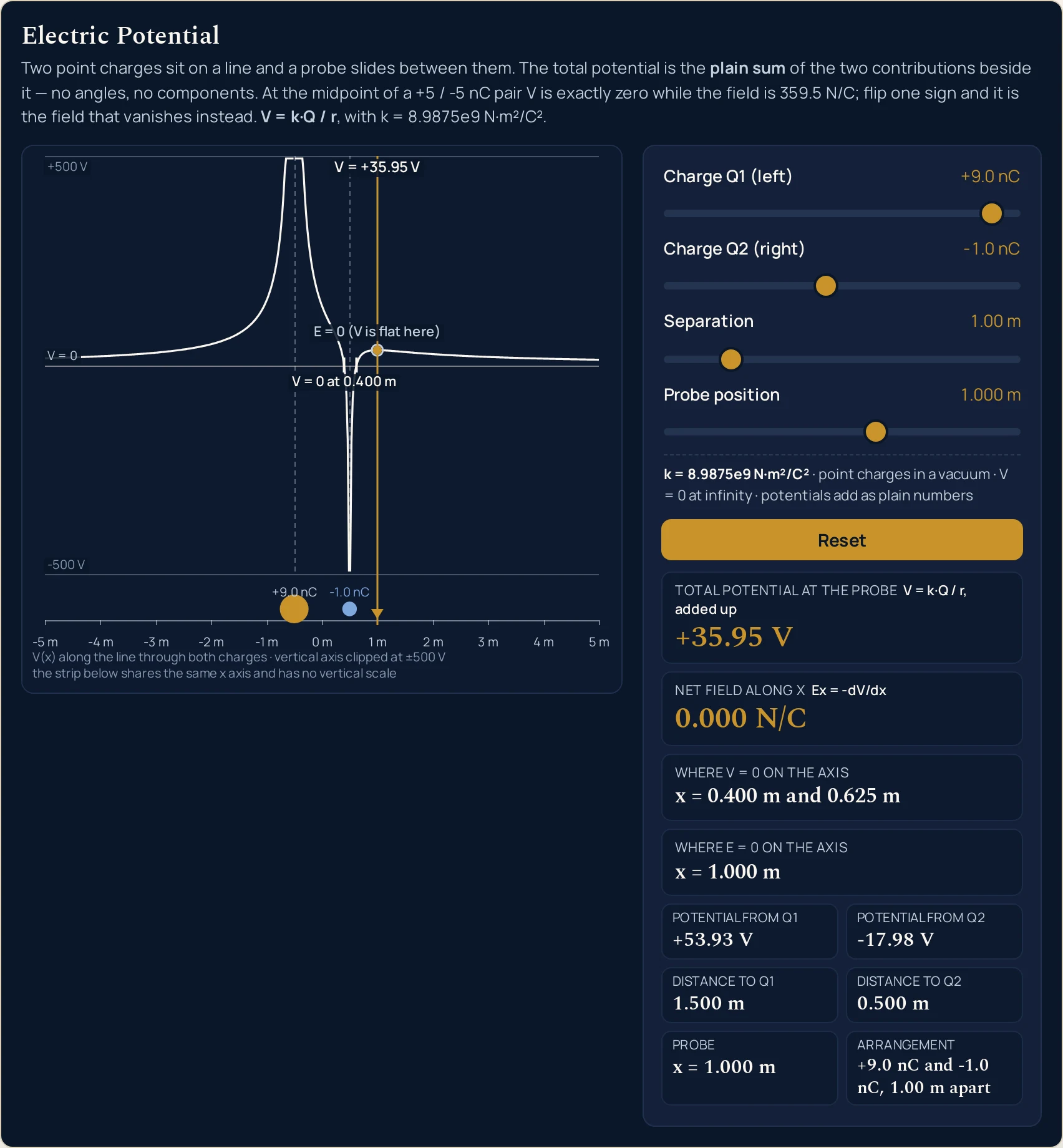
- Load the unequal pair and separate the three special points. With +9.0 nC and -1.0 nC, 1.00 m apart the cards read x = 0.400 m and 0.625 m for the potential and x = 1.000 m for the field, three different places on one axis. Park the probe on each in turn and read the other card as you go.
- Press Reset when you have lost the thread. It returns the two charges to +5.0 nC and -5.0 nC, the separation to 1.00 m and the probe to x = 0.000 m, and replays the settle so the curve slides back into place rather than jumping. The panel then reads the first row of the table below.
- Read the fixed line last of all. It says k = 8.9875e9 N·m²/C² · point charges in a vacuum · V = 0 at infinity · potentials add as plain numbers. That is the whole of what this panel assumes, in one line, and it is worth copying down beside any figure you take away from here.
If typing suits you better than dragging — or if you want the relation run backwards, so that a potential and a charge give back the distance that produces it — that is the job of the electric potential calculator, which also takes microcoulombs and centimetres these sliders have no menu for. For what the potential actually is, why its zero sits at infinity, and seven problems worked end to end, read the full guide to electric potential.
Worked example: change one thing at a time
Every row below is one setting of the four sliders, and every cell is a string the running lab printed there. The ten settings are the ones this cluster publishes, so they are also the ones the lab’s own tests pin. Where a cell and the panel ever part company, the panel is right.
| Arrangement | Probe | Total potential | Net field along the axis | Where V is zero | Where the field is zero |
|---|---|---|---|---|---|
| +5.0 nC and -5.0 nC, 1.00 m apart | x = 0.000 m | 0.000 V | +359.5 N/C | x = 0.000 m | nowhere on the axis |
| +5.0 nC and -5.0 nC, 1.00 m apart | x = 0.250 m | -119.8 V | +798.9 N/C | x = 0.000 m | nowhere on the axis |
| +5.0 nC and -5.0 nC, 1.00 m apart | x = -0.500 m | — | — | x = 0.000 m | nowhere on the axis |
| +5.0 nC and -5.0 nC, 4.00 m apart | x = 0.000 m | 0.000 V | +22.47 N/C | x = 0.000 m | nowhere on the axis |
| +5.0 nC and +5.0 nC, 1.00 m apart | x = 0.000 m | +179.8 V | 0.000 N/C | nowhere on the axis | x = 0.000 m |
| +5.0 nC and +5.0 nC, 1.00 m apart | x = 0.200 m | +214.0 V | -407.6 N/C | nowhere on the axis | x = 0.000 m |
| +9.0 nC and -1.0 nC, 1.00 m apart | x = 0.400 m | 0.000 V | +998.6 N/C | x = 0.400 m and 0.625 m | x = 1.000 m |
| +9.0 nC and -1.0 nC, 1.00 m apart | x = 0.625 m | 0.000 V | -511.3 N/C | x = 0.400 m and 0.625 m | x = 1.000 m |
| +9.0 nC and -1.0 nC, 1.00 m apart | x = 1.000 m | +35.95 V | 0.000 N/C | x = 0.400 m and 0.625 m | x = 1.000 m |
| +1.0 nC and 0.0 nC, 1.00 m apart | x = 0.000 m | +17.98 V | +35.95 N/C | nowhere on the axis | nowhere on the axis |
Rows 1 and 5 are the pair to read first. They are the same two charges half a metre either side of the same probe, differing in one sign. Row 1 reads 0.000 V with a field of +359.5 N/C; row 5 reads +179.8 V with a field of 0.000 N/C. Exactly one of the two quantities is zero in each row, and it is the other one each time — because the two field contributions point the same way in row 1 and opposite ways in row 5, which is the side of the picture the electric field simulator draws as arrows.
Rows 1 and 4 change only the separation. The potential card prints the identical string 0.000 V at both, while the field falls from +359.5 N/C to +22.47 N/C as the charges go from 1.00 m to 4.00 m apart — a factor of sixteen, for four times the distance in an inverse-square quantity. Pulling a dipole apart weakens its field at the midpoint and leaves the zero of its potential exactly where it was.
Rows 7, 8 and 9 are one arrangement with the probe in three places. The last two columns are identical down all three, because they describe the charges rather than the probe. What changes is where the probe is standing: at x = 0.400 m the potential is zero and the field is +998.6 N/C, at x = 0.625 m the potential is zero again and the field has reversed to -511.3 N/C, and at x = 1.000 m the field is 0.000 N/C while the potential is +35.95 V.
Row 3 is the row with no numbers in it. The probe sits exactly on the left-hand charge, and two of the six columns print an em dash rather than an enormous number. The last two columns carry on, because they never asked where the probe was.
The same ten settings, with the sum shown
The table above gives the answers; this one gives the two numbers they were made from. Read the third and fourth columns here against the third column above and superposition stops being a word.
| Arrangement | Probe | Potential from Q1 | Potential from Q2 | Distance to Q1 | Distance to Q2 |
|---|---|---|---|---|---|
| +5.0 nC and -5.0 nC, 1.00 m apart | x = 0.000 m | +89.88 V | -89.88 V | 0.500 m | 0.500 m |
| +5.0 nC and -5.0 nC, 1.00 m apart | x = 0.250 m | +59.92 V | -179.8 V | 0.750 m | 0.250 m |
| +5.0 nC and -5.0 nC, 1.00 m apart | x = -0.500 m | — | — | — | — |
| +5.0 nC and -5.0 nC, 4.00 m apart | x = 0.000 m | +22.47 V | -22.47 V | 2.000 m | 2.000 m |
| +5.0 nC and +5.0 nC, 1.00 m apart | x = 0.000 m | +89.88 V | +89.88 V | 0.500 m | 0.500 m |
| +5.0 nC and +5.0 nC, 1.00 m apart | x = 0.200 m | +64.20 V | +149.8 V | 0.700 m | 0.300 m |
| +9.0 nC and -1.0 nC, 1.00 m apart | x = 0.400 m | +89.88 V | -89.88 V | 0.900 m | 0.100 m |
| +9.0 nC and -1.0 nC, 1.00 m apart | x = 0.625 m | +71.90 V | -71.90 V | 1.125 m | 0.125 m |
| +9.0 nC and -1.0 nC, 1.00 m apart | x = 1.000 m | +53.93 V | -17.98 V | 1.500 m | 0.500 m |
| +1.0 nC and 0.0 nC, 1.00 m apart | x = 0.000 m | +17.98 V | 0.000 V | 0.500 m | 0.500 m |
Row 1 is +89.88 V and -89.88 V from 0.500 m each way, and the card above prints their sum as 0.000 V. Row 5 is +89.88 V twice over from the same two distances, and the card prints +179.8 V. One sign is the entire difference between the two results, and no geometry was needed to get from the cells to the card in either case.
One coincidence in this table is worth noticing and not worth building on. Row 7 prints +89.88 V and -89.88 V, the same pair of strings as row 1, from 0.900 m and 0.100 m rather than half a metre each way — nine nanocoulombs far off against one nanocoulomb close to. The two rows are not the same situation and the cards beneath them differ completely. Two equal-looking readings can come from arrangements that have nothing else in common.
Row 10 is the degenerate case the lab still handles. The second charge is turned down to 0.0 nC, which the cell prints without a sign, and its contribution reads 0.000 V while the distance cell carries on reporting 0.500 m. A single charge has no place on the axis where its potential vanishes and no place where its field does, so both of the bottom cards read nowhere on the axis at once.
Formula and symbol reference
The panel prints its two relations on itself, inside the labels of the cards they feed. V = k·Q / r, added up sits above the total potential and Ex = -dV/dx sits above the net field, so neither answer arrives without the rule that produced it. Neither is derived here.
The first of those is the whole of what the lab computes, applied twice and added. The second is a statement about the picture rather than a calculation the panel performs: the field along the axis is the slope of the curve drawn above it, which is why the marked point where the field vanishes sits exactly where the curve goes flat. The constant that scales both of them, 8.9875e9, is the one set out by the guide to Coulomb’s law, and it is on the fixed line so that no figure here arrives without it.
| Symbol | Meaning | SI unit | In this lab |
|---|---|---|---|
| Q1 | Charge on the left of the pair, set by the Charge Q1 (left) slider. Its sign decides whether it raises or lowers the potential everywhere around it | coulomb (the slider is in nanocoulombs) | -10 to +10 in steps of 0.1, printed to one decimal with a sign in the cell beside the slider: “+5.0 nC”, “+9.0 nC”, “+1.0 nC”. |
| Q2 | Charge on the right of the pair, set by the Charge Q2 (right) slider. Turning it to zero leaves a single charge on the axis and the lab keeps working | coulomb (the slider is in nanocoulombs) | the same -10 to +10 in steps of 0.1: “-5.0 nC”, “+5.0 nC”, “-1.0 nC”, and exactly “0.0 nC” with no sign at the middle. |
| d | Separation between the two charges, on the Separation slider. They always sit at half of it either side of the origin, so this is the only control that moves them | metre | 0.4 to 4 in steps of 0.05, printed to two decimals: “1.00 m” on the default pair and “4.00 m” at the far stop. |
| x | Position of the probe, on the Probe position slider — and also the horizontal axis of the entire drawing, which is fixed and does not rescale | metre | -5 to +5 in steps of 0.005, printed to three decimals: “0.000 m”, “0.250 m”, “0.625 m”, “-0.500 m”. |
| V | Total potential at the probe, on the first card. A scalar: one signed number, no direction, and the plain sum of the two cells below it | volt | four significant figures with a sign: “+179.8 V”, “-119.8 V”, “+35.95 V”, and an unsigned “0.000 V” when the two contributions cancel. |
| Ex | Net field along the axis at the probe, on the second card. The card label prints the relation it applies, Ex = -dV/dx, rather than leaving it to be assumed |
newton per coulomb | four significant figures with a sign: “+998.6 N/C” at one zero of V, “-511.3 N/C” at the other, and “0.000 N/C” at a null point. |
| V1 and V2 | What each charge contributes on its own, in the Potential from Q1 and Potential from Q2 cells. Their sum is the card above, every time | volt | four significant figures with a sign: “+89.88 V” against “-89.88 V” at the dipole midpoint, “+53.93 V” against “-17.98 V” at the null point. |
| r1 and r2 | Distance from the probe to each charge, in the Distance to Q1 and Distance to Q2 cells. Each one is what the charge above it was divided by | metre | three decimals: “0.500 m”, “0.100 m”, “1.125 m”, “2.000 m” — and an em dash when the probe is on a charge. |
| k | The Coulomb constant, which the fixed line under the sliders prints rather than hiding. It is the one number on the panel you cannot change | newton metre squared per coulomb squared | a constant: 8.9875e9, written exactly that way on the fixed line, and the value this site’s electric field calculator already uses. |
The row worth reading twice is the probe position. Its step of 0.005 m is not a taste in round numbers: x = 0.625 m is one of the two places the potential vanishes on the unequal pair, and a coarser grid would put that position out of reach of the slider altogether. The charge and separation steps are chosen the same way, so that every setting published on this page lands exactly rather than being snapped to a neighbour.
The physics: why potentials add as plain numbers
Everything on the left of the screen hangs on one decision: there is a single horizontal scale, position along the axis in metres, and it is fixed from -5 to +5 m whatever the sliders say. Nothing is drawn at a place that scale did not put it — not the charges, not the probe, not the zero marks, not the tick labels. That is what makes two screenshots of this lab comparable at a glance.
The upper region, about three-quarters of the height, is the potential plotted against that scale, and it is the part that earns the lab its point. The two contributions are added before anything is drawn, so the curve is the total and not a pair of curves overlaid. Where it crosses the zero line the lab puts a cream tick and writes the position out; where it goes flat it marks the point and labels it E = 0 (V is flat here).
That flat spot is the honest version of the second card. The field along a line is the slope of the potential along it, so a place where the curve levels off is a place where the field has nothing left to push with — even though the potential there is nowhere near zero. On the unequal pair that point sits at x = 1.000 m, half a metre beyond the smaller charge, and the card beside it still reads +35.95 V.
The curve has to be clipped, because it runs away at each charge. The lab chooses a limit from the arrangement rather than a fixed one, draws a dashed vertical line where each asymptote is, and prints the limit in the caption: vertical axis clipped at ±200 V on the default pair, and a different figure on a different arrangement. A drawing that truncated its own axis without saying so would be misleading in exactly the way a caption is meant to prevent.
Where the field belongs in all this is one line and no more: it falls one power of distance faster than the potential does, which is why the two quantities can vanish in different places at all. Its direction, its lines and its inverse-square law are the subject of the electric field guide and are not worked out anywhere on this page. This lab borrows a single number from it, prints it on a card, and stops.
Narrow the browser and the drawing gives things up in a settled order rather than shrinking everything towards illegibility. The charge labels shorten and then drop, the metre-tick ladder stops rather than skipping a rung, and the caption gives up its lines from the last one upwards, so the line naming the clip is the one it always keeps. Every label that is drawn over the curve is painted on a small plate of background colour first, so the curve can never be mistaken for a stroke through a word.
One consequence of that ordering is visible on the unequal pair. Its two zero crossings are less than a quarter of a metre apart, and at most widths there is room for one label between them, so the lab draws both ticks and labels the first. The card in the panel prints both positions in full, x = 0.400 m and 0.625 m, which is the division of labour the whole page runs on: the picture shows where, the panel says exactly where.

Where the electric potential simulator breaks down
The lab solves its own model exactly, so nothing on the screen ever fails. Everything below is a limit of that model, of the slider grid, or of what a one-dimensional drawing can carry, and each item says what this lab does about it.
- These are point charges, and nothing real is one
- The relation the panel applies is exact for charge concentrated at a mathematical point, and it stays exact outside any spherically symmetric charge — a shell, a uniformly charged ball or a charged sphere — with the distance measured from the centre. Inside a shell or a conductor it is simply wrong: the potential stops climbing and levels off instead of running away. The dashed asymptotes this lab draws at each charge are therefore a feature of the idealisation and not of any object, and no reading taken closer to a charge than a real object’s own radius describes anything.
- Everything here lives on one line, and the zeros are the zeros on that line
- The set of points where the potential of two opposite charges vanishes is a surface, and the axis this lab draws cuts through it at the positions the card names. The card says on the axis for that reason and never says anywhere. The same caution applies to the field: nowhere on the axis means nowhere along this one line, which is a smaller claim than it looks. A contour map would make the point better and is the article’s job, not this panel’s.
- The zero of potential is a choice, so a negative reading is about that choice
- This lab puts zero infinitely far from both charges, which is the convention that makes the relation come out with nothing added to it, and the fixed line says so. It is not the only choice available: a car takes its chassis as zero and a house takes the earth. A card reading -119.8 V means the probe is below the zero this lab picked, and nothing more than that. Only differences in potential move energy about, which is why the choice is free in the first place.
- Nothing here moves, and nothing here responds
- The two charges are held where the sliders put them, with no forces acting and no history. There are no conductors anywhere in the picture, so there is no induced charge, no earthed surface rearranging itself as the probe approaches, and no dielectric. Put the same pair in water rather than vacuum and every potential on the panel would shrink by a large factor; there is no permittivity control, so a reading taken in a medium needs dividing before it means anything.
- The constant on the fixed line is rounded, and not everywhere the same way
- This lab prints 8.9875e9, the value chosen so that the potential tools and the field tools of this cluster agree digit for digit. The measured value carries further digits, and the Coulomb law calculator on this site rounds it to 8.988e9 instead. All of them agree to four significant figures and part company in the digit after that, so a number carried from one page to another may not survive its last digit. Do not read the fourth figure of any reading here as though it were measured.
- The vertical axis is clipped, and the caption is the only place that says by how much
- Near a charge the curve leaves the top or bottom of the plot, and what you see there is the plot’s edge rather than the potential’s value. The limit is chosen from the arrangement, so it changes when you change the charges or the separation: the default pair clips at 200 V and the unequal pair at 500 V. Read the caption of the drawing in front of you, not the caption of a screenshot taken somewhere else.
- The axis stops at five metres either side, and it does not rescale
- Holding the scale fixed is what makes every arrangement comparable, and the price is that a feature further out than five metres is not drawn. Widely separated unequal charges can put their outer zero past that edge, in which case the picture has nothing to mark and the caption notes it. The panel is unaffected either way: the cards work from the arithmetic, not from what happened to fit in the frame.
- The sliders move on a grid, so some positions are unreachable
- The probe steps in 0.005 m, the charges in 0.1 nC and the separation in 0.05 m. Every setting this page publishes lands exactly on that grid, which is why it was chosen, but a position between two steps cannot be dialled in at all — the browser snaps it to a neighbour before the lab ever sees it. If you need an arbitrary distance or an arbitrary charge, type it into the calculator instead of chasing it with a slider.
- Do not rebuild one reading out of two others
- Every figure is computed from the exact value and rounded once for display, so a chain of rounded readings need not close. Row 2 is the clearest case: the two contribution cells print +59.92 V and -179.8 V, whose difference is 119.88, while the card above them prints -119.8 V. Neither is wrong and neither was rounded twice. Take each reading from the cell that publishes it, and treat any figure you rebuild as approximate.
- Nothing here has been measured
- Four slider positions go in and one idealised arrangement comes out. No reading on this page describes a real object, a real charge or a real laboratory, and a preset name is only a label for the four values it writes. The lab is a place to see a relation behave, not a source of data. Check anything you intend to depend on against a source of your own before you quote it.
Where electric potential is actually used
- Settling the “zero potential means zero field” argument in one click
- This is the misconception the lab was built to end, and it takes two presets and no arithmetic. Load Dipole: V is zero, the field is not, read 0.000 V beside +359.5 N/C, then load Like charges: the field is zero, V is not and read +179.8 V beside 0.000 N/C. The same two charges, one sign apart, and each time it is the other quantity that vanishes.
- Checking a superposition answer before trusting it
- Set the two charges and the separation you were given, park the probe where the question asks, and compare the card against the two cells under it. If your own arithmetic disagrees with Total potential at the probe but matches one of the contributions, you dropped the other term; if it disagrees with both, you have a unit or a sign wrong. The distances are printed too, so there is no step of the working the panel leaves you to guess at.
- Finding a null point before doing the algebra
- The closed form for the place where two fields cancel is easy to misremember and easy to sign-slip. Dial in the charges and read Where E = 0 on the axis, which gives the answer without the probe being anywhere near it, and only then work it out by hand to see whether you agree. On +9.0 nC and -1.0 nC, 1.00 m apart it is at x = 1.000 m, outside the smaller charge rather than between the two.
- Showing a class what a scalar buys them
- Put the probe anywhere off centre, at x = 0.250 m say, and the panel gives +59.92 V, -179.8 V and a total of -119.8 V. Ask the room to do the same for the field and the answer needs directions before it needs numbers. Doing both sums on the same screen, for the same two charges, is a faster argument for the scalar than any amount of saying so.
- Reading a curve as a landscape
- The plot is a height map along a line, and the field is its gradient, so a student can be asked where a released positive charge would roll before any formula is written down. Flat means no push, steep means a hard one, and downhill means the direction. The marked point labelled E = 0 (V is flat here) is where that reading of the picture and the second card agree in front of you.
- Seeing why a chosen zero is a convention and not a measurement
- Load One charge on its own and watch both bottom cards read nowhere on the axis together. A single positive charge never reaches zero potential anywhere at a finite distance, so the zero this lab reports is the one it declared at infinity rather than a place it found. That is precisely the same move an engineer makes when a chassis or an earth pin is called zero volts, which the potential difference guide takes up from the circuit end.
- Auditing a sign before anything else
- The commonest error in this topic is a lost minus. Set the charge you were handed, put the probe at the distance you were given, and look only at whether the card is above or below zero: a positive charge raises the potential everywhere around it and a negative one lowers it everywhere, at every distance, with no exceptions. If a quoted answer has the wrong side of zero, nothing further in the working is worth checking.
Where to go next
The topic itself — what the potential is, why it is a scalar, what an equipotential surface is, why the zero sits at infinity and a set of problems worked end to end — is in the electric potential guide. If typing suits you better than dragging, the electric potential calculator heads the list below and runs the same relation in all three directions.
The neighbouring questions have tools of their own. The electric field guide with its simulator covers the vector half of this picture; the guide to Coulomb’s law with its lab covers the force two charges exert on each other and where the constant comes from; and the potential difference guide covers the same volt arrived at from a circuit.
Further out, the guide to electric charge is where the nanocoulomb on these sliders comes from, the capacitance guide treats the ratio of charge to potential as a quantity in its own right, and the potential energy guide is the mechanical cousin of the same idea. The rest is in the library of physics simulations and on the blog.
Frequently asked questions
Why does the potential card read 0.000 V at the midpoint when there is plainly a field there?
Because the two cards answer different questions, and separating them is what this lab is for. Potential is a plain sum of signed numbers: the +89.88 V from the positive charge and the -89.88 V from the negative one cancel exactly. The field is a sum of directions, and at that point both charges push a positive test charge the same way, so the two contributions reinforce instead of cancelling. The field card reads +359.5 N/C.
I dragged the probe from one end of the axis to the other and the Where V = 0 card never changed. Is it stuck?
No, and that is the cleanest single check in the lab. Where the potential vanishes is a property of the two charges and their separation, never of where the probe is standing. Load Two places where V vanishes and then drag the probe wherever you like: the card holds at x = 0.400 m and 0.625 m every time, and Where E = 0 holds at x = 1.000 m beside it.
Why do six readouts turn into a dash when the probe sits on a charge?
Because the potential of an idealised point charge is undefined at zero distance, not merely large. Put the probe at x = -0.500 m on the default arrangement and the total potential, the net field, both contributions and both distances all print an em dash. The two cards that describe the arrangement carry on: Where V = 0 still reads x = 0.000 m, because it never depended on the probe.
Can the potential really be negative, or is a minus sign there a mistake?
It is real, and it is a statement about where zero was put rather than about a shortage of anything. This lab takes the potential to be zero infinitely far from both charges, which is the usual convention and the one that makes the formula come out with nothing added to it. A negative reading means that point sits below the chosen zero. Drag the probe towards the negative charge and watch the card fall through it.
Why does the caption say the vertical axis has been clipped?
Because the curve runs away to infinity at each charge, so an honest plot has to stop somewhere and say where. The lab picks a limit from the arrangement itself, draws a dashed line at each charge, and prints the limit it used. On the default pair the caption reads vertical axis clipped at ±200 V; switch to the unequal pair and the same caption reads ±500 V instead.
What exactly is the point where the field is zero but the potential is not?
It is the place on the axis where the two fields cancel while the two potentials do not. Load The null point, where V is 35.95 V: the probe sits at x = 1.000 m on a +9.0 nC and -1.0 nC pair, the field card reads 0.000 N/C and the potential card reads +35.95 V. On the curve it is the flat spot, because the field is the slope of the potential.
Why does the probe slider step in 0.005 m rather than something rounder?
Because one of the lab’s own published positions is x = 0.625 m, the outer place where the potential vanishes on the +9.0 nC and -1.0 nC pair. A step of 0.01 would put that position off the grid and the browser would snap it to 0.62 or 0.63. The charge sliders step in 0.1 nC and the separation in 0.05 m for the same reason: every published setting has to land exactly.
Does this lab find all the places where the potential is zero?
No, only the places on the line it draws, and the cards say so in as many words. Around two opposite charges the set of points at zero potential is a surface, and the axis merely cuts through it at the positions the card names. Everything in this simulation lives on one line, which is why the two cards end with on the axis and why there is no contour map anywhere in it.
References & formula source
- One constant drives every number on this panel, and the lab prints it on a fixed line under the sliders rather than hiding it: k = 8.9875e9 N·m²/C², with the three assumptions beside it — point charges in a vacuum, the potential taken as zero infinitely far away, and potentials added as plain numbers. That value is the one this site’s electric field calculator already uses, adopted here so that V = k·Q / r and the inverse-square field relation agree digit for digit across the cluster. The 2019 SI redefinition released the magnetic constant, so this one is measured rather than defined: CODATA 2022 gives 8.9875517862e9, uncertain by 14 in the last two digits quoted, and the familiar 8.9875517873681764e9 is the value k held by definition before that change. Our Coulomb law calculator rounds the constant to 8.988e9 instead, and the panel’s 8.9875e9, that rounding and the measured value all agree to four significant figures and part company in the digit after that.
- Potentials add as plain signed numbers because the potential is a scalar. The total at a point is the sum of k·Q / r taken over the charges, each term carrying the sign of its own charge and no direction whatsoever, and that single sum is the whole of the physics behind the first card. The two contribution cells beside it exist so the addition can be watched rather than believed. The field card performs a different kind of sum, one that is one-dimensional here only because every object in this lab sits on the same line.
- The positions the two zero cards name come from closed forms that this cluster derived and then re-checked numerically over a hundred arrangements rather than trusting on their own. For two charges of opposite sign the potential vanishes once between them, and a second time outside the smaller charge when the magnitudes differ; for two charges of the same sign it vanishes nowhere on the axis at all. The field vanishes between two like charges, outside the smaller of two unlike ones, and nowhere for an equal and opposite pair — which is why the dipole preset reads nowhere on the axis in the fourth card.
- Every headline zero here is exact in the physics and about 1e-14 V in floating point, because it is a difference of two numbers near a hundred. The lab prints 0.000 V rather than a long tail of arithmetic noise at precisely the moment a reader is told the answer is zero, and it decides that relative to the size of the terms that cancelled rather than against a fixed threshold. A snapped zero is always printed without a sign, so a reading of minus nought point nought nought nought never appears.
- A probe at zero distance from a charge returns nothing rather than a number. Six readouts blank to an em dash, and no reading anywhere in this lab can become an infinity or a not-a-number whatever the sliders are set to. The case of two equal and opposite charges, where the formula for an off-centre null point would divide by zero, is settled before the division rather than repaired after it, and the fourth card simply says there is no such point on the axis.
- Every reading quoted on this page is a string the simulation itself printed at the four slider positions named beside it, read back out of the running lab rather than worked out by hand. Each figure is computed from the exact value and rounded once for display, so rebuilding one printed number out of two others will not always land on the same last digit — take each reading from the cell that publishes it. Where anything written here and the panel ever disagree, the panel is the one to believe, and any figure you mean to depend on deserves checking against a source of your own first.
- Further reading: Electric potential — Wikipedia