A conductivity figure tells you how much heat a wall will pass once it has settled. It says nothing about the wait, and the wait is what this lab draws: the temperature right through a slab while the heat is still arriving, against the dashed straight line it is heading for. The quantity that sets the pace is the thermal diffusivity, α = k/(ρc), and five sliders let you build that quantity out of a conductivity, a density and a specific heat capacity, choose a thickness, and then run the clock it implies.
Thermal Diffusivity: How Fast the Heat Actually Gets Through
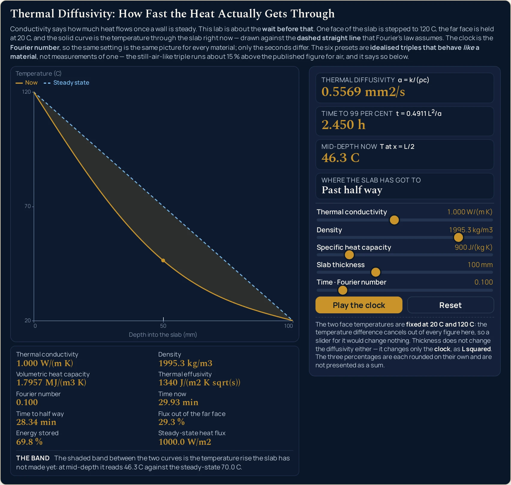
Conductivity says how much heat flows once a wall is steady. This lab is about the wait before that. One face of the slab is stepped to 120 C, the far face is held at 20 C, and the solid curve is the temperature through the slab right now — drawn against the dashed straight line that Fourier's law assumes. The clock is the Fourier number, so the same setting is the same picture for every material; only the seconds differ. The six presets are idealised triples that behave like a material, not measurements of one — the still-air-like triple runs about 15 % above the published figure for air, and it says so below.
Thermal conductivity1.000 W/(m K)
Density1995.3 kg/m3
Volumetric heat capacity1.7957 MJ/(m3 K)
Thermal effusivity1340 J/(m2 K sqrt(s))
Fourier number0.100
Time now29.93 min
Time to half way28.34 min
Flux out of the far face29.3 %
Energy stored69.8 %
Steady-state heat flux1000.0 W/m2
The bandThe shaded band between the two curves is the temperature rise the slab has not made yet: at mid-depth it reads 46.3 C against the steady-state 70.0 C.
Thermal diffusivity α = k/(ρc)
0.5569 mm2/s
Time to 99 per cent t = 0.4911 L2/α
2.450 h
Mid-depth now T at x = L/2
46.3 C
Where the slab has got to
Past half way
Thermal conductivity1.000 W/(m K)
Density1995.3 kg/m3
Specific heat capacity900 J/(kg K)
Slab thickness100 mm
Time · Fourier number0.100
The two face temperatures are fixed at 20 C and 120 C: the temperature difference cancels out of every figure here, so a slider for it would change nothing. Thickness does not change the diffusivity either — it changes only the clock, as L squared. The three percentages are each rounded on their own and are not presented as a sum.
Load a real case on the sliders
Each button presses the lab's own Reset and then writes all five sliders, so every load starts from the same place and a running clock is stopped before the new values land. Work down the list and watch the Thermal diffusivity card and the Time to 99 per cent card disagree about which material is the interesting one. Every name ends in -like for a reason, set out where the limits of the model are.
Pick a case above, or drag the five sliders yourself.
What Is the Thermal Diffusivity Simulator?
The thermal diffusivity simulator is a free interactive physics lab that runs in your browser, with nothing to install and no sign-up. It draws the temperature right through a slab while the heat is still arriving: a solid curve for where the slab has got to, a dashed straight line for the steady state it is heading for, and a shaded band between them for the temperature rise still to come.
Five sliders set the thermal conductivity from 0.010 to 398.107 W/(m K), the density from 1.0 to 10000.0 kg/m3, the specific heat capacity from 100 to 5000 J/(kg K), the slab thickness from 5 to 300 mm and the clock, which is the dimensionless Fourier number, from 0 to 0.80.
Four cards answer with the thermal diffusivity alpha = k/(rho c) in square millimetres per second, the time the slab needs to reach 99 per cent of its steady state, the temperature at mid-depth now, and one of three phrases saying where the slab has got to.
Ten smaller cells carry the conductivity, density and volumetric heat capacity you set, the effusivity built from them, the clock in both dimensionless and real form, the time to half way, the flux leaving the far face and the energy stored as percentages of their settled values, and the steady-state heat flux. Play the clock runs time forward; Reset restores 1.000 W/(m K), 1995.3 kg/m3, 900 J/(kg K), 100 mm and a Fourier number of 0.100.
| Control | Range | Step |
|---|---|---|
| Thermal conductivity | 0.010 to 398.107 W/(m K) | logarithmic, 0.02 |
| Density | 1.0 to 10000.0 kg/m3 | logarithmic, 0.02 |
| Specific heat capacity | 100 to 5000 J/(kg K) | 5 J/(kg K) |
| Slab thickness | 5 to 300 mm | 5 mm |
| Fourier number | 0 to 0.80 | 0.002 |
How to use the thermal diffusivity simulator
- Start from the state it opens in. The lab boots at rest on 1.000 W/(m K), 1995.3 kg/m3, 900 J/(kg K), 100 mm and a clock reading of 0.100, so every card is already filled before you touch anything. Reset returns all five sliders to exactly that and stops the clock if it is running.
- Set the conductivity. Thermal conductivity is logarithmic, because the quantity spans four orders of magnitude between a still gas and a metal, and a linear slider from 0.010 to 398.107 would squeeze every insulator into the first hundredth of its travel. The card beside it always prints the conductivity itself, never the exponent: 0.010 W/(m K) at one end, 398.107 W/(m K) at the other. Fourier's law of thermal conduction is where that quantity comes from and what it does once the wall is steady.
- Set the density and the specific heat capacity. Density is logarithmic for the same reason; Specific heat capacity is linear, from 100 to 5000 J/(kg K) in steps of 5. These two reach the answer only as their product, which the panel prints for you as Volumetric heat capacity in MJ/(m3 K).
- Set the thickness. Slab thickness runs from 5 to 300 mm in steps of 5 and is the one slider that leaves every material card exactly where it was. What it moves is the clock: the time to 99 per cent goes from 22.0 s at 5 mm to 22.046 h at 300 mm for the same brick-like triple.
- Move the clock. Time · Fourier number runs from 0 to 0.80 in steps of 0.002. It is dimensionless on purpose, so the same reading is the same picture for every material; Time now gives you that instant in seconds, minutes, hours or days beside it.
- Read the four cards down the right. Thermal diffusivity carries its own formula line,
α = k/(ρc), to four decimal places at every size. Time to 99 per cent and Mid-depth now sit under it, and Where the slab has got to prints one of exactly three phrases: Still filling, Past half way, Practically steady. - Read the ten cells under the graph. The three material figures you set, the effusivity built from them, the clock in both forms, the two times, and then the two percentages that matter most: Flux out of the far face and Energy stored, each against its own settled value. Steady-state heat flux closes the row with the figure a conduction calculation would have given you all along.
- Read the sentence strip headed The band. It describes the shading between the two curves, and it changes its mind when there is nothing left to shade. Below a Fourier number of 0.558 it names the gap at mid-depth; at and above it, it says that no band is drawn.
- Press Play the clock to let it run. The clock advances at 0.08 in the Fourier number every second and the button becomes Pause the clock while it is going. Only the clock moves; the three material sliders and the thickness stay exactly where you put them.
If the wall has already settled and all you want is the rate through it, this is more lab than you need. The Fourier's law lab draws the straight line on its own, with the area and the temperature difference that go with it, and that straight line is the dashed one here. Come back the moment the question turns into how long.
Worked example: change one thing at a time
Every row below is one setting of the five sliders, and every cell is a string the running lab printed there. The first six are the presets; the next four hold the brick-like triple still and walk the clock from its first step to its last; the final two change nothing but the thickness. Where a cell and the lab ever part company, believe the lab.
| Setting | Sliders, as the panel reads them | Thermal diffusivity | Time to 99 per cent | Mid-depth now | Where the slab has got to | Time now | Flux out of the far face | Energy stored |
|---|---|---|---|---|---|---|---|---|
| A brick-like wall | 1.000 W/(m K) · 1995.3 kg/m3 · 900 J/(kg K) · 100 mm · 0.100 | 0.5569 mm2/s | 2.450 h | 46.3 C | Past half way | 29.93 min | 29.3 % | 69.8 % |
| A copper-like bar | 398.107 W/(m K) · 9120.1 kg/m3 · 385 J/(kg K) · 100 mm · 0.492 | 113.3807 mm2/s | 43.3 s | 69.5 C | Practically steady | 43.4 s | 98.4 % | 99.4 % |
| A stainless-like plate | 15.136 W/(m K) · 7943.3 kg/m3 · 500 J/(kg K) · 100 mm · 0.096 | 3.8109 mm2/s | 21.48 min | 45.3 C | Past half way | 4.20 min | 26.9 % | 68.6 % |
| A still-air-like gap | 0.026 W/(m K) · 1.2 kg/m3 · 1005 J/(kg K) · 100 mm · 0.300 | 21.7688 mm2/s | 3.76 min | 66.7 C | Past half way | 2.30 min | 89.6 % | 95.8 % |
| A water-like layer | 0.603 W/(m K) · 1000.0 kg/m3 · 4185 J/(kg K) · 100 mm · 0.300 | 0.1440 mm2/s | 9.474 h | 66.7 C | Past half way | 5.788 h | 89.6 % | 95.8 % |
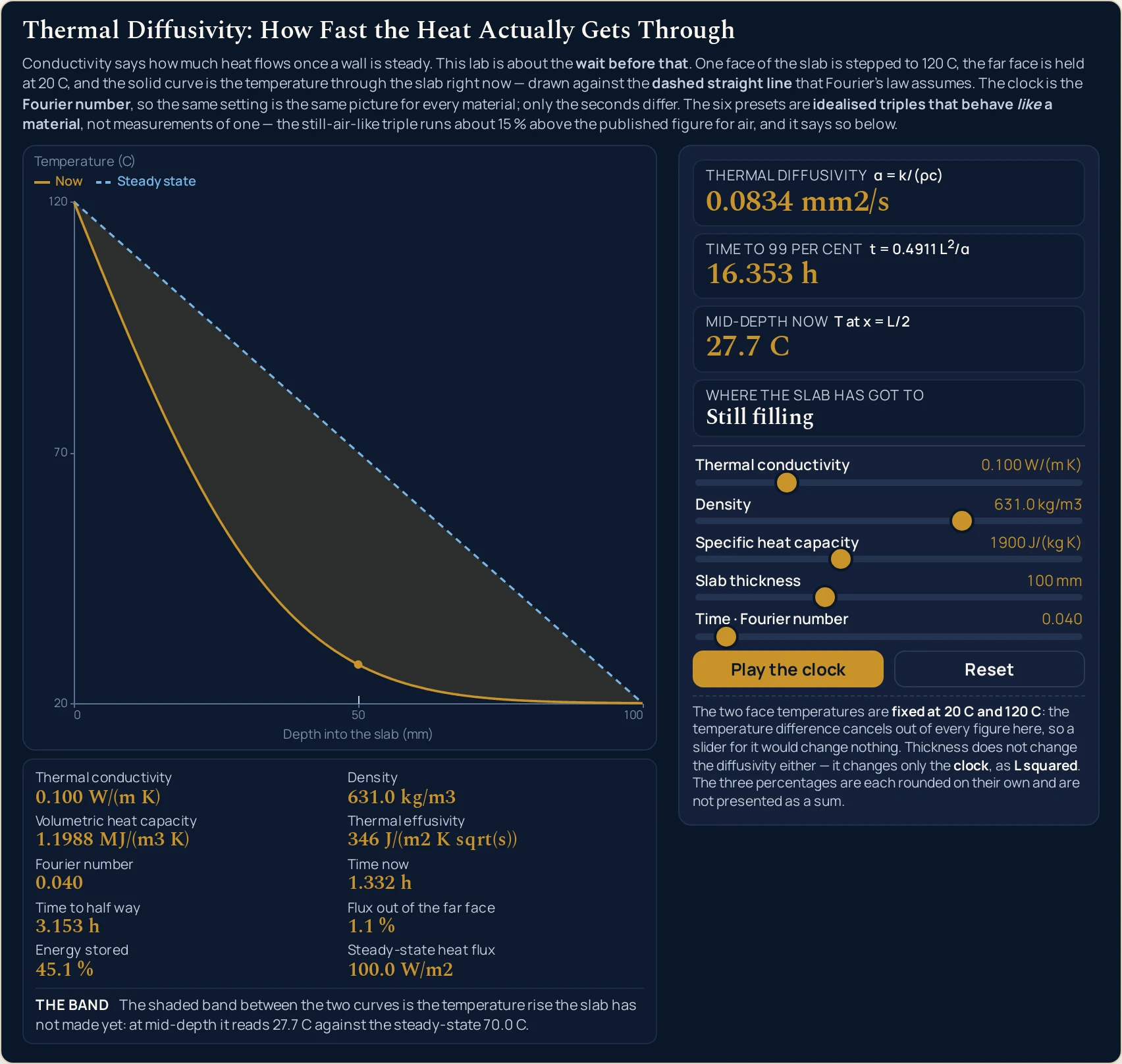
| A pine-like board | 0.100 W/(m K) · 631.0 kg/m3 · 1900 J/(kg K) · 100 mm · 0.040 | 0.0834 mm2/s | 16.353 h | 27.7 C | Still filling | 1.332 h | 1.1 % | 45.1 % |
| Brick-like, first clock step | 1.000 W/(m K) · 1995.3 kg/m3 · 900 J/(kg K) · 100 mm · 0.002 | 0.5569 mm2/s | 2.450 h | 20.0 C | Still filling | 35.9 s | 0.0 % | 10.1 % |
| Brick-like, just past half way | 1.000 W/(m K) · 1995.3 kg/m3 · 900 J/(kg K) · 100 mm · 0.096 | 0.5569 mm2/s | 2.450 h | 45.3 C | Past half way | 28.73 min | 26.9 % | 68.6 % |
| Brick-like, practically steady | 1.000 W/(m K) · 1995.3 kg/m3 · 900 J/(kg K) · 100 mm · 0.492 | 0.5569 mm2/s | 2.450 h | 69.5 C | Practically steady | 2.454 h | 98.4 % | 99.4 % |
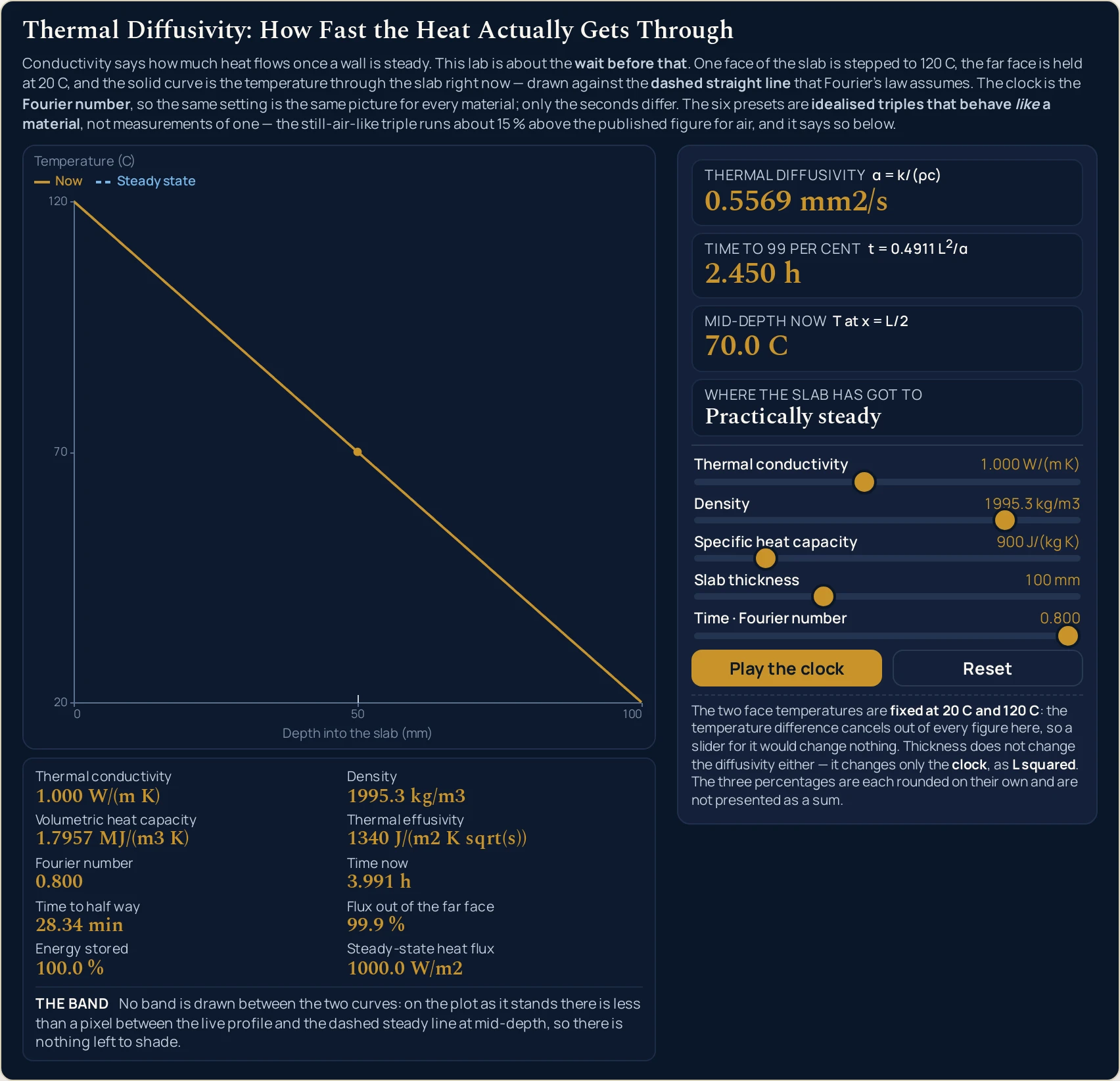
| Brick-like, far right edge | 1.000 W/(m K) · 1995.3 kg/m3 · 900 J/(kg K) · 100 mm · 0.800 | 0.5569 mm2/s | 2.450 h | 70.0 C | Practically steady | 3.991 h | 99.9 % | 100.0 % |
| Brick-like, 25 mm thin | 1.000 W/(m K) · 1995.3 kg/m3 · 900 J/(kg K) · 25 mm · 0.100 | 0.5569 mm2/s | 9.19 min | 46.3 C | Past half way | 1.87 min | 29.3 % | 69.8 % |
| Brick-like, 300 mm thick | 1.000 W/(m K) · 1995.3 kg/m3 · 900 J/(kg K) · 300 mm · 0.100 | 0.5569 mm2/s | 22.046 h | 46.3 C | Past half way | 4.489 h | 29.3 % | 69.8 % |
Rows 3 and 4 are the pair the lab exists for. The stainless-like plate conducts about 575 times better than the still-air-like gap, and the gap still diffuses a temperature change 5.71 times faster, at 21.7688 mm2/s against 3.8109. Both ratios come from the unrounded triples the sliders hold rather than from the rounded cards. A steady-state tool has nowhere to put a density or a specific heat, so it can never show you that inversion.
Rows 4 and 5 print the same temperatures on purpose. The still-air-like gap and the water-like layer both sit at a clock reading of 0.300, so both give Mid-depth now 66.7 C, Flux out of the far face 89.6 % and Energy stored 95.8 %, to the last digit. That is the whole point of a dimensionless clock, and it is not a copied row: the two differ by a factor of about 151 in real time, 3.76 min against 9.474 h.
Rows 7 to 10 hold one material still and move only the clock. The diffusivity and the time to 99 per cent print the same strings in all four, because neither depends on where the clock stands. What moves is the picture: 20.0 C at the first step, then 45.3, then 69.5, then 70.0 C, which is exactly the steady-state midpoint of the two fixed faces. The Energy stored column climbs 10.1, 68.6, 99.4, 100.0 per cent behind it.
Rows 1, 11 and 12 are the geometry lesson. Same material, same clock reading, the same temperature picture to the last digit — only the time moves, and it moves as the thickness squared: 9.19 min at 25 mm, 2.450 h at 100 mm and 22.046 h at 300 mm, which are ratios of exactly 16 and 9. If you would rather type a published triple than dial one in on a logarithmic slider, the thermal diffusivity calculator takes the same relation to more figures and runs it backwards for the conductivity, the density or the specific heat.
Formula and symbol reference
The lab works from one definition and one dimensionless group. The diffusivity is α = k/(ρc), and the clock is the Fourier number Fo = αt/L2, which is the only combination of material, time and thickness the temperature profile cares about. Everything else on the panel is that profile read at a particular depth, or the same clock read at a particular threshold.
The density and the specific heat capacity appear only as their product, so halving one and doubling the other leaves the diffusivity exactly where it was. That is algebra, not a discovery, and nothing here tests it: specific heat capacity is defined per kilogram while what conduction cares about is per cubic metre, and the density is simply the bridge between them.
| Symbol | Meaning | SI unit | In this lab |
|---|---|---|---|
| α | Thermal diffusivity: how fast a temperature change travels through the material. The headline card, and the only quantity here that answers how soon | square metre per second, m2/s | Printed in mm2/s to four decimal places at every size, with no magnitude switch: “0.5569 mm2/s” on the opening state, “0.0056 mm2/s” at the bottom of the conductivity slider and “1111.1111 mm2/s” at the bottom of the density slider. |
| k | Thermal conductivity: how much heat crosses a metre of the material per kelvin, once nothing is changing any more. The numerator of the diffusivity | watt per metre per kelvin, W/(m K) | The slider is logarithmic and steps in hundredths of the exponent, so the card runs from “0.010 W/(m K)” to “398.107 W/(m K)”. It reads “1.000 W/(m K)” after Reset. |
| ρ | Density. It never acts alone in this lab: it enters only multiplied by the specific heat capacity | kilogram per cubic metre, kg/m3 | Logarithmic as well, in hundredths of the exponent: “1.0 kg/m3” at the bottom, “10000.0 kg/m3” at the top, “1995.3 kg/m3” after Reset. The far ends take the diffusivity to “1111.1111 mm2/s” and “0.1111 mm2/s”. |
| c | Specific heat capacity: the energy it takes to raise a kilogram of the material by one kelvin | joule per kilogram per kelvin, J/(kg K) | 100 to 5000 in steps of 5; “900 J/(kg K)” after Reset. Taken alone to either end the diffusivity reads “5.0119 mm2/s” and “0.1002 mm2/s”, and the time to 99 per cent runs from “16.33 min” to “13.609 h”. |
| ρc | Volumetric heat capacity, the product of the two above. The denominator of the diffusivity, and the whole of what those two sliders contribute | joule per cubic metre per kelvin, J/(m3 K) | Printed in MJ/(m3 K) to four decimal places: “1.7957 MJ/(m3 K)” after Reset, “0.0009 MJ/(m3 K)” with the density slider at its bottom stop and “9.9763 MJ/(m3 K)” with the specific heat slider at its top one. |
| L | Slab thickness. It is not a material property and it changes no material card — it sets the clock those cards are measured against | metre, m; the lab works in millimetres | 5 to 300 mm in steps of 5; “100 mm” after Reset. The diffusivity does not move across that whole range; the time to 99 per cent goes from “22.0 s” to “22.046 h” and the steady-state flux from “20000.0 W/m2” to “333.3 W/m2”. |
| Fo | The Fourier number, and the clock this lab runs on. One dimensionless group that carries the whole transient, so the same value is the same picture for every material | none — it is a ratio | 0 to 0.80 in steps of 0.002, printed to three decimal places; “0.100” after Reset. The thresholds behind the status card sit at 0.0946870 and 0.4910769, between slider stops rather than on one. |
| t | The same instant in real time, printed as Time now so you never have to do the conversion yourself | second, s | Chooses its own unit from the figure it is about to print: “0.0 s” at the left-hand end of the clock, “29.93 min” after Reset, “3.991 h” at the right-hand end of the clock, and “2.08 d” with the conductivity slider taken to its bottom stop. |
| t50 | Time to half way: how long mid-depth takes to make half of its final rise. Printed as Time to half way | second, s | “28.34 min” after Reset. It is a fixed fraction of the time to 99 per cent for every material, because both are the same clock read at two thresholds: “8.4 s” for the copper-like bar, “3.153 h” for the pine-like board. |
| t99 | Time to 99 per cent, from t = 0.4911 L2/α. The headline answer to “how long until this has settled?” |
second, s | “2.450 h” on the opening 100 mm wall, “9.19 min” at 25 mm and “22.046 h” at 300 mm — the same material three times, with the thickness squared doing all of it. |
| e | Thermal effusivity, e = sqrt(k × ρ × c). The same three properties arranged the other way round, and the one that decides the first instant of contact rather than the hours after it |
J/(m2 K sqrt(s)) | Whole numbers: “1340” after Reset, “37388” for the copper-like bar, “346” for the pine-like board and “6” for the still-air-like gap. |
| T at L/2 | The temperature at mid-depth right now, printed as Mid-depth now. The reading the two thresholds are defined against | kelvin, K; the lab prints degrees Celsius | One decimal place, between the two fixed face temperatures: “20.0 C” with the clock at zero, “46.3 C” after Reset and “70.0 C” at the right-hand end, which is exactly the steady-state midpoint of 20 and 120. |
| q | Steady-state heat flux: what will cross the slab per square metre once it has settled. Printed as Steady-state heat flux | watt per square metre, W/m2 | One decimal place: “1000.0 W/m2” after Reset, “26.3 W/m2” for the still-air-like gap and “398107.2 W/m2” for the copper-like bar. It depends on the conductivity and the thickness, and not at all on the clock. |
| q/q at rest | Flux out of the far face as a percentage of that steady value. What the far face is delivering now, as against what it will deliver once the slab has settled | none — it is a percentage | One decimal place, from “0.0 %” at the left-hand end of the clock to “99.9 %” at the right. It reads “98.4 %” at the instant the status card turns to Practically steady. |
| U/U at rest | Energy stored in the slab as a percentage of the energy it will hold when steady. Printed as Energy stored | none — it is a percentage | One decimal place: “69.8 %” after Reset, “10.1 %” one clock step off zero, and “100.0 %” at the right-hand end of the clock. |
Two of those rows are worth a second look. The Thermal diffusivity card keeps four decimal places from 0.0056 right up to 1111.1111, with no switch to fewer digits anywhere in between, which is deliberate: a magnitude branch is exactly where a rounding bug hides. And Thermal effusivity is printed as a whole number, which is honest at 37388 and lossy at 6 — a point the section below returns to.
The physics: why the profile bends before it straightens
Heat arriving at the hot face has two jobs, and every joule does one or the other. Some of it presses on into the material ahead; the rest is spent lifting the temperature of the material already behind it. The first is what the conductivity measures and the second is what the volumetric heat capacity measures, so the front advances at the rate the one outruns the other.
That is what the bend in the gold curve is. The dashed line is the state Fourier's law assumes, a straight fall from the hot face to the cold one; the solid curve is where the slab has actually got to; and the band between them is the temperature rise the slab has not made yet, because the heat that would have made it is still being absorbed on the way. As the absorption finishes, the curve straightens onto the line.
Mid-depth is 99 per cent of the way there at a Fourier number of 0.4911, which for a given slab is t = 0.4911 L2/α. The thickness enters squared, and the three brick-like rows of the table above show it doing so exactly: a quarter of the thickness gives a sixteenth of the wait, three times the thickness gives nine times. Nothing else in the relation can produce a factor like that.
Ninety-nine per cent in temperature is not ninety-nine per cent in everything. At the clock reading where the status card turns over, mid-depth has made 99 per cent of its rise, but Flux out of the far face reads 98.4 % and Energy stored reads 99.4 %. Temperature settles before the flux does, and the lab prints all three so you can see them disagree. The full account of thermal diffusivity works the constants through with diagrams and problems.
The constant 0.4911 is exact algebra for this threshold, because the mid-depth series contains only odd terms and the next one after the first is smaller than any arithmetic here can see. The companion figure for the far face is a solved root rather than a closed form, and it is the larger of the two. Both belong to one arrangement only: a slab that starts uniform, one face stepped, the far face held.
The status card is thresholded on the clock, not on the temperature beside it. The two thresholds are solved from the same series the curve is drawn from, and both land between slider stops rather than on one, so the phrase cannot flicker. The table below reads the stops either side of each, and adds the stop where the shading gives up.
| Clock reading | Where the slab has got to | Mid-depth now | Flux out of the far face | The band |
|---|---|---|---|---|
| 0.094 | Still filling | 44.8 C | 25.8 % | drawn |
| 0.096 | Past half way | 45.3 C | 26.9 % | drawn |
| 0.490 | Past half way | 69.5 C | 98.4 % | drawn |
| 0.492 | Practically steady | 69.5 C | 98.4 % | drawn |
| 0.556 | Practically steady | 69.7 C | 99.2 % | drawn |
| 0.558 | Practically steady | 69.7 C | 99.2 % | not drawn |
Rows 3 and 4 are the interesting pair. The card changes from Past half way to Practically steady while Mid-depth now prints 69.5 C at both and the flux column does not move either. Nothing physical happened at that stop; a threshold on the clock was crossed, and the reading beside it had already rounded to its final value.
The band stops being drawn at a clock reading of 0.558. That is a pixel test on the plot the lab is actually drawing, not a statement about the physics: this canvas gives a plot 381 px tall at every column width, and at 0.558 the two curves are closer together than one pixel at mid-depth. The figure belongs to that plot. An independent check on a nominal 300 px plot puts the same test at 0.534, and the two are not interchangeable — a taller plot keeps the curves apart for longer.
Where the slab model breaks down
The lab solves its own model exactly, so nothing on the screen ever fails. Everything below is a limit of that model, of the situation it stands for, or of the way the figures are printed, and each item says what the lab does about it.
- The hot face steps instantly, and nothing real does
- At the first instant the model puts a 100 K jump across zero thickness, so the flux into that face is formally infinite and the profile there is vertical. A real surface is warmed through an air film, a contact resistance or a joint, all of which delay the whole picture by an amount this lab knows nothing about. Thin, fast layers suffer most from it, because their own clock is short enough for the delay to matter.
- The three material figures are held constant
- Conductivity, density and specific heat capacity all move with temperature, and the diffusivity inherits every one of those movements. Over a small range the drawing is fine; across a quench or a furnace it is not. Post 713 lists k is a fixed constant for each material among its misconceptions, and this is the same point seen from the transient side: run the lab at both ends of your range and treat the two answers as a band.
- One dimension, two faces, no edges
- Heat here flows straight through the slab and nowhere else. A corner, a stud bridging an insulated cavity or a pipe buried in a floor is a two- or three-dimensional problem, and the front arrives sooner than this drawing says because it has more than one route. There is no control for it, because the model has no term for it.
- Nothing convects and nothing radiates
- Both faces are held at fixed temperatures rather than exchanging heat with air or with a surrounding surface. A real far face loses heat to a room and so never quite reaches a fixed value, and the still-air-like preset is the worst case of the lot, because a real air gap circulates rather than merely conducting and this model has no term for that. The comparison of conduction, convection and radiation sets out what the other two do.
- The three Fourier constants are not universal
- The two thresholds behind the status card, 0.0946870 and 0.4910769, and the far-face figure that goes with them, belong to this boundary condition alone: uniform to start with, one face stepped, the other held for ever. Heat the slab from both sides, insulate its back face, or make it a rod or a sphere, and the same thickness-squared law carries a different number in front of it. The diffusivity does not change; only the schedule does.
- The presets are idealised triples, not materials
- Each is chosen to land near a published diffusivity and each lands a little off it: brick-like is 7.1 per cent high against 0.52 mm2/s, copper-like 2.1 per cent high against 111, stainless-like 9.3 per cent low against 4.2, water-like 0.7 per cent high against 0.143, pine-like 1.7 per cent high against 0.082, and the still-air-like gap 14.6 per cent high against 19. The air gap is the big one, and it is printed here rather than quietly closed by tuning the triple.
- Dividing one printed figure by another will not always come out
- Every card is rounded on its own and the arithmetic behind it is not. Thermal effusivity is the clearest case: it reads 7753 for the stainless-like plate and 6 for the still-air-like gap, and dividing those gives about 1292, while the unrounded triples behind them give 1375. The one-significant-figure card is carrying the whole of that error, which is why this page quotes 1375 and names where it came from.
- Two readings that agree are sometimes only one reading
- The Volumetric heat capacity cell and the Thermal diffusivity card are the same arithmetic seen twice, since the card is simply the conductivity divided by that cell. Their agreeing is a definition restated and proves nothing about the material. The same goes for the temperature difference: it cancels out of the clock, the times and every percentage, which is why there is no slider for it.
- Nothing here has been measured
- The five sliders are things you chose, and no reading on this page describes a particular wall, bar or board. The lab will happily draw a 300 mm slab of something ten times denser than steel with the specific heat of water. Whether such a thing exists is a separate question the arithmetic has no view on, so check any figure you intend to rely on against your own data first.
Where the diffusivity clock is actually used
- Heavy walls that lag the afternoon
- Load the brick-like wall and drag the thickness to 300 mm: Time to 99 per cent reads 22.046 h, which is most of a day, while the material cards do not move at all. That lag is why a thick stone building stays cool through a hot afternoon, and it is set by the diffusivity and the thickness rather than by the conductivity on its own. The steady-state account of the same wall names the effect and hands the quantity over; this is the quantity.
- Deciding when a test rig has actually settled
- A measurement that assumes steady conduction is wrong until the transient has finished, and the two are easy to confuse because the temperature stops moving first. Run the clock up and watch Flux out of the far face reach 98.4 % at the very stop where the card first says Practically steady. On the brick-like wall that is 2.454 h after the step, against a Time now of 29.93 min at the state the lab opens in.
- Why a cavity fills quickly and still insulates
- The still-air-like gap reaches 99 per cent of its steady state in 3.76 min, behind only the copper-like bar among these six, and its Steady-state heat flux is 26.3 W/m2 against 1000.0 for the brick-like wall. Filling fast and passing little are not in conflict: there is almost nothing in a gas to warm up, and almost nothing to carry heat either. It is the clearest case on these sliders of why the two quantities answer different questions.
- Comparing two materials on the same clock
- Set any two triples to the same Fourier number and the profiles are identical, so the comparison you are left with is the one that matters: how long each took. That is the discipline the dimensionless clock enforces, and it is why Time now sits beside Fourier number rather than replacing it. Use the specific heat calculator if the figure you are missing is the one under the line.
- Sanity-checking a published diffusivity
- A handbook may give you a conductivity, a density and a specific heat but no diffusivity, or a diffusivity and no triple. Dial in whichever three you have and compare the card with the published figure: the gap is real information about the sample, the temperature or the table. Every preset here is 0.7 to 14.6 per cent away from its published value, and none of them was tuned to close that gap.
- Teaching how much against how soon
- Load the still-air-like gap and then the stainless-like plate and the two readings go opposite ways, which is the inversion rows 3 and 4 of the table above set out in figures: the far better conductor is the slower diffuser. That is hard to believe on paper and immediate here, because one press of a preset moves both readings at once. The heat transfer lab puts conduction beside convection and radiation once the idea has landed.
Where to go next
For the quantity in full, with worked problems, the three questions one material answers differently and the diagrams that go with them, read Thermal Diffusivity: How Fast Heat Moves. If you would rather type your own conductivity, density and specific heat than dial them in, the calculator is the first card under Related tools below, and it will run the relation backwards for whichever of the three you are missing.
The steady state this transient ends in belongs to Fourier's Law of Thermal Conduction, which carries the conductivity table, R-value, U-value and layers in series, with the Fourier's law lab and the thermal conduction calculator beside it. For the quantity under the line there is Specific Heat Capacity, the specific heat lab and the specific heat calculator.
Further afield, Conduction, Convection and Radiation covers the two mechanisms this model leaves out, Heat vs Temperature separates the energy from the reading, and Thermal Expansion Explained and its lab take up what the temperature change does to size. The rest of the collection is in the library of physics simulations and on the blog, and the site search will find a topic by name.
Frequently asked questions
What does this thermal diffusivity simulator actually show?
It draws the temperature right through a slab while that slab is still warming up. The dashed straight line is the steady state Fourier's law assumes; the solid curve is where the slab has got to; the shaded band between them is the temperature rise it has not made yet. On the state the lab opens in, mid-depth reads 46.3 C against a steady-state 70.0 C.
Why is the clock a Fourier number instead of seconds?
Because the same Fourier number is the same picture for every material, which is the whole point of the lab. Set the clock to 0.100 and the profile looks identical whether the slab is brick-like or air-like; only the time it took differs. Time now converts it for you: 29.93 min for the brick-like wall, 45.9 s for the still-air-like gap.
Why do two different materials print exactly the same temperatures?
Because they are at the same point on the clock. The still-air-like gap and the water-like layer both sit at a Fourier number of 0.300, so both print Mid-depth now 66.7 C and Flux out of the far face 89.6 per cent. Nothing is wrong. They differ only in how long that took: Time to 99 per cent reads 3.76 min against 9.474 h.
When does the shaded band disappear?
At a Fourier number of 0.558, on the plot this lab actually draws. The rule is a pixel test rather than a physics test: once the live curve and the dashed line are within one pixel of each other at mid-depth, the band is switched off and the sentence under the graph says so instead of pretending there is still something to see.
Why does the card change to Practically steady while the temperature reading stays put?
Because the card is thresholded on the clock, not on the rounded temperature. At a Fourier number of 0.490 the card reads Past half way and at 0.492 it reads Practically steady, while Mid-depth now prints 69.5 C at both. The threshold is solved from the same series the curve is drawn from, so it lands between two slider stops and cannot flicker.
Can I dial a real material into these sliders?
Not exactly, which is why every preset name ends in -like. Each one is an idealised triple of conductivity, density and specific heat chosen to land near a published diffusivity, and each lands a little off it: the still-air-like gap comes out 14.6 per cent above the published figure for air. Type your own figures into the thermal diffusivity calculator when they have to be yours.
What exactly is the time to 99 per cent?
It is the time mid-depth takes to reach 99 per cent of its final rise, for one particular arrangement: a slab that starts uniform, with one face stepped and the far face held for ever. That gives t = 0.4911 L squared divided by alpha. Heat the slab from both sides or insulate its back and the constant in front changes, so the figure does not carry across.
Why is there no slider for the temperature difference?
Because it would change nothing you can read. The two faces are fixed at 20 C and 120 C, and the temperature difference cancels out of the Fourier number, the times and every percentage on the panel. That is algebra rather than something the lab discovers, and it is why the vertical axis can stay fixed and the profiles stay comparable between settings.
Is the thermal diffusivity the same as the thermal conductivity?
No, and the presets are laid out so you can watch them disagree. The still-air-like gap conducts about 575 times worse than the stainless-like plate, and diffuses a temperature change 5.71 times faster, because the diffusivity divides the conductivity by the volumetric heat capacity. Conductivity answers how much heat finally flows; diffusivity answers how soon the change arrives.
References & formula source
- Carslaw and Jaeger, Conduction of Heat in Solids: the separation-of-variables solution for a slab held between two fixed face temperatures, which is the series this lab evaluates at every setting of its sliders.
- Incropera and DeWitt, Fundamentals of Heat and Mass Transfer: the Fourier number as the dimensionless clock of a transient, and the conditions under which a one-term form of the series is good enough.
- Wikipedia, "Thermal diffusivity", retrieved 21 September 2026: every published diffusivity quoted on this page - copper 111, air 19, stainless steel 304A 4.2, brick 0.52, water 0.143 and yellow pine 0.082 mm2/s - comes from its table of selected materials, and none of them was measured here.
- Each of the three Fourier constants this page names belongs to one boundary condition only: a slab that starts uniform, with one face stepped to a new temperature and the far face held at the old one for ever. A slab heated from both faces, or one with an insulated back, settles on a different schedule.
- Every figure on this page is a reading this simulation printed for a setting of its own five sliders. The six triples are idealised values chosen to land near a published diffusivity, not measurements of any particular brick, bar or board, so verify anything you intend to rely on against your own data before use.
- Further reading: Thermal diffusivity — Wikipedia