A block of rock 100 km across, a source at its left edge and a recording station at its right, and two wavefronts that set off together. This p-wave speed simulator is a free interactive lab that races them across it and prints what the slider positions imply: a P-wave speed of 5773.50 m/s, an S-wave speed of 3333.33 m/s, a speed ratio of 1.7321 and an S-wave that arrives 12.68 s later.
Drag Shear modulus G down and the gap between the fronts widens; take it to zero and the S-front is not drawn at all, while the P-front still crosses at 4303.31 m/s. That is the difference between a wave slowing down and a wave ceasing to exist, and it is what this picture exists to make unmissable.
P-Wave Speed
Set the rock's stiffness and density and race the two body waves across it. The P-wave carries the P-wave modulus M = K + 4G/3 and travels at vp = sqrt(M / ρ); the S-wave carries only the shear modulus and travels at vs = sqrt(G / ρ). Because 4G/3 is always bigger than G, the P-wave is always first — that is what the P stands for. Drag the shear modulus to zero and the S-front does not slow down, it disappears: a liquid has nothing to shear.
Load a real rock
Each button presses the lab’s own Reset first and then writes the four sliders, so every press starts from the same known state and re-runs the race. Every number you then see is the lab’s own, and the line underneath quotes the cards back to you.
The first three hold the distance at 100 km and move the material; the last two are deliberate extremes, and only one of them is a rock. All five sets of figures are stated givens chosen to make a point.
Pick a rock above, or drag the sliders yourself.
What Is the P-Wave Speed Simulator?
The p-wave speed simulator is a free interactive physics lab that runs in your browser, with nothing to install and no sign-up. It draws a block of rock in cross-section with a seismic source at its left edge and a recording station at its right, and races two wavefronts across it: a P-front, drawn as a band of compressed and rarefied lines, and behind it an S-front, drawn as a sideways wiggle. The picture comes to rest at the instant the P-front reaches the station, so the gap the S-front still has to cover is the head start, drawn as a dashed span and labelled with it.
Four sliders drive it, each printing its own setting beside its name. Bulk modulus K runs 0 to 120 GPa in steps of 1 and opens at 50; Shear modulus G runs 0 to 80 GPa in steps of 1 and opens at 30. Density runs 1000 to 4000 kg/m3 in steps of 50 and opens at 2700, and Distance to the station runs 10 to 500 km in steps of 10 and opens at 100.
Four cards carry the answer, each with its own relation printed beside the label. The headline is the P-wave speed to two decimals, and under it sit the S-wave speed, the speed ratio to four decimals and how much later the S-wave arrives. At the opening setting those read 5773.50 m/s, 3333.33 m/s, 1.7321 and 12.68 s.
The shear modulus is the slider that makes this lab worth opening, and dragging it is the fastest way to see why a compression wave cares about a material resisting a change of shape. Take it from 30 to 15 GPa and the two speeds fall to 5091.75 and 2357.02 m/s while the ratio widens to 2.1602, so the S-wave is 22.79 s late instead of 12.68 s. Take it to 0 and the P-wave speed falls to 4303.31 m/s, a factor of 0.74536, which is exactly sqrt(5/9) at these figures.
At a shear modulus of zero the S-front is not drawn at all, and that is the result rather than a failure. The S-wave speed card prints an exact 0.00 m/s, and the speed ratio and the lag both print no S-wave rather than an infinity: a liquid has nothing to shear, so there is no slow S-wave, there is none. Approach the endpoint instead of landing on it and everything stays finite - at G = 1 GPa the S-wave card reads 608.58 m/s and the ratio 7.1647.
Both moduli at zero is refused for a different reason, and the lab says which. With nothing to carry a wave at all there is no speed to report - not a slow one, and not a zero - so every speed-derived reading changes to no medium, the S-wave card included. The P-wave modulus cell still prints 0.00 GPa, because that modulus really is zero and printing it is what makes the refusal legible rather than mysterious.
A compact grid under the cards holds six more readings. It gives the P-wave modulus K + 4G/3 in GPa, Poisson's ratio to four decimals and signed, the two arrival times in seconds, the P-wave speed again in km/s for comparing with published figures, and a fixed cell holding the ratio floor, sqrt(4/3) = 1.1547. That last cell is a bound rather than a state, so no slider moves it and it still prints 1.1547 when everything else reads no medium.
Poisson's ratio is the cell to watch beside the speed ratio, because it fixes that ratio on its own. At the opening figures it is exactly 0.2500, which is the only reason the ratio is exactly sqrt(3); it is exactly 0.5000 whenever the shear modulus is zero, and exactly -1.0000 whenever the bulk modulus is. So the sqrt(3) is a condition and not a fact about rock, and the panel lets you break it with one drag.
The fourth slider is the only one that is not a property of the material, and it moves nothing but the clock. Distance to the station drives the two arrival cells, the lag card and the station label in the drawing, and leaves both speeds exactly where they were. Over the same rock the lag runs 1.27 s at 10 km, 12.68 s at 100 km and 63.40 s at 500 km - exactly linear in the distance, because the head start is bought at a fixed rate per kilometre.
A caption strip under the drawing names which of four cases is on screen and explains it in a sentence: solid rock, no shear stiffness - no S-wave, limiting case - no resistance to compression for a bulk modulus of zero, and no medium. Two further standing lines state the things the picture must not be read against: that the P-wave is faster than the S-wave for every physical rock, that the ratio has a floor, and that the moduli are gigapascals on screen and pascals inside the formula, a factor of 1e9 the lab applies for you.
The drawing is honest about what it is and is not drawing. The two fronts share one distance scale - the S-front is placed at the P-front's distance divided by the computed speed ratio at every instant - so the drawn gap is the real head start and the caption can say the P-front has run 1.7321x further. The sideways wiggle on the S-front is schematic and its height carries no quantity, which the lab states under the scene: there is no amplitude control and no amplitude card, so the wiggle can never be read as a measurement.
What the lab leaves out, stated as omissions rather than as assumptions that happen to hold. It draws the isotropic, homogeneous, non-attenuating case, so the fronts are flat and nothing refracts, reflects, splits or decays, while real ground is layered, cracked and faster along the bedding than across it. It has no frequency, no wavelength and no amplitude, and it runs the clock forwards only - it cannot turn a measured arrival gap back into a distance. Nothing on the panel is a measurement: the three material properties are stated givens, never properties attributed to a named rock, so verify any figure against your own source before you use it for anything that matters.
| Control | Range | Step, default and what it moves |
|---|---|---|
| Bulk modulus K | 0 to 120 GPa | steps of 1 GPa, opening on 50, where the read-back beside the slider says "50 GPa". It is the stiffness against being squeezed smaller, and it is in the P-wave speed only - the S-wave card does not react to it at all. Zero is a legal setting and the last preset uses it: the speed ratio then sits on its exact floor of 1.1547 and Poisson's ratio reads exactly -1.0000, the theoretical lower bound, which the caption strip names as a limiting case rather than a rock. With the shear modulus at zero as well, every speed-derived reading prints "no medium" instead of a number |
| Shear modulus G | 0 to 80 GPa | steps of 1 GPa, opening on 30, where the read-back says "30 GPa". This is the slider worth dragging: it is in BOTH speeds, so both rise with it at every one of its 81 positions while the speed ratio falls and Poisson's ratio falls with it. Zero is legal and meaningful rather than an error - the S-front is then not drawn at all, the S-wave card prints an exact 0.00 m/s, and the speed ratio and the lag print "no S-wave" rather than an infinity, while the P-wave card still prints 4303.31 m/s. A shear modulus just above zero keeps every reading finite |
| Density of the rock | 1000 to 4000 kg/m³ | steps of 50 kg/m³, opening on 2700, where the read-back says "2700 kg/m3". It is the inertia term, so both speeds fall together as the rock gets heavier - 9486.83 m/s at the light end down to 4743.42 m/s at the heavy one, at the opening moduli. The speed ratio does not move at all across that range, holding at 1.7321, because the density divides out of it. The panel prints it as "Density rho" and takes it as a stated given, never as a property of a named rock |
| Distance to the station | 10 to 500 km | steps of 10 km, opening on 100, where the read-back says "100 km". It is the only control that is not a property of the material, and it moves nothing but the clock: the two arrival cells, the lag card and the station label in the drawing. Neither speed card changes by a digit. The lag is exactly linear in it - 1.27 s over 10 km, 12.68 s over 100 km, 25.36 s over 200 km and 63.40 s over 500 km - which is the half of this topic the companion calculator has no box for |
| Replay and Reset | two buttons | the first is labelled "Replay" and re-runs the race from the source with the rock unchanged, over about a second and a quarter. The second is labelled "Reset" and restores every default AND replays, which is why all five of the landing page's preset payloads press it before writing the sliders. Neither button changes its label and neither carries a pressed state, because there is no mode on this lab. There is no pause control either: the picture eases to its new state and then stops, so there is no running animation to stop |
How to use the p-wave speed simulator
- Read the four cards before you touch anything. They are already answering for the opening rock: P-wave speed
5773.50 m/s, S-wave speed3333.33 m/s, Speed ratio1.7321and S-wave arrives later by12.68 s. Each carries its own relation beside the label, so you can see which formula produced which number. - Find the two fronts in the drawing. The
Pmarker has reached the station; theSmarker is still short of it, and the dashed span between them is labelled12.68 s behind. That gap is the whole subject of this lab, which is why the picture rests at the P-wave’s arrival rather than running on. - Drag Shear modulus G and watch four things move at once. Both speed cards fall, the speed ratio rises, and the S-marker slides back towards the source. At
15 GPathey read5091.75 m/s,2357.02 m/s,2.1602and a lag of22.79 s— nearly double the opening wait. - Take that slider all the way to
0 GPa, which is where most of the value is. The S-front disappears from the drawing entirely. The S-wave speed card prints an exact0.00 m/s, the ratio and the lag both printno S-wave, and the P-wave card still prints4303.31 m/s. A liquid has nothing to shear, so there is no slow S-wave — there is none. - Now drag Bulk modulus K to zero as well. Every speed-derived reading changes to
no medium, the S-wave card included, and no front is drawn. The P-wave modulus cell still reads0.00 GPa, which is the lab showing you why it refused rather than leaving you guessing. - Put the shear modulus back to
30 GPaand leave the bulk modulus at zero. This is the fourth case and the oddest: the ratio card lands on1.1547, exactly the fixed floor cell under it, the two fronts almost touch at a lag of4.02 s, and Poisson’s ratio reads an exact-1.0000. No real rock sits there. - Drag Density and notice what does not move. Both speeds fall together as the rock gets heavier —
9486.83 m/sat1000 kg/m3down to4743.42 m/sat4000— and the speed ratio holds at1.7321the whole way, because the density divides out of it. - Drag Distance to the station and notice that neither speed changes at all. A distance is in neither formula. It moves the two arrival cells, the lag card and the
station 100 kmlabel in the drawing:1.27 sof lag over10 km,63.40 sover500 km. - Read the compact grid under the cards. It gives the P-wave modulus, Poisson’s ratio, the two arrival times, the P-wave speed again in km/s for comparing with published figures, and a ratio floor cell fixed at
1.1547that no slider can move. - Press Replay to run the race again with the rock unchanged, and Reset when you have finished. Reset restores every default and replays, so you always land back on
50 GPa,30 GPa,2700 kg/m3and100 km— the state every figure on this page is measured against.
Dragging is the right way to find out which readings move together and a poor way to land on a particular state, because the shear slider alone has 81 positions. The five preset buttons above exist for that, and the P-wave guide is where the subject itself is argued from scratch, with the shear term derived and eight problems worked step by step.
What this panel cannot do is run either relation backwards. It only ever goes forwards, from three material sliders to two speeds, so a question that hands you a speed and asks for a modulus or a density needs the P-wave speed calculator, which solves in four directions and prints the working for each.
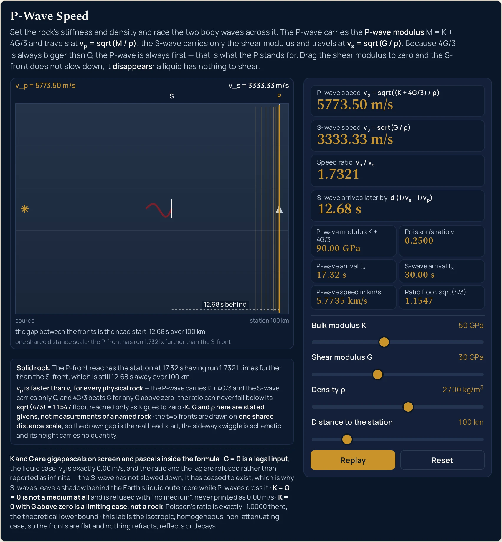
12.68 s short of it. The ratio card reads 1.7321 and the dashed span is drawn to match — the P-front really is measured 1.7321 times further from the source. The band in the drawing writes v_p in ASCII, because a canvas has no markup to draw a subscript with.Worked example: change one thing at a time
Nothing in the three tables below was worked out here. Each row is a state the lab was put into through its own sliders and then read back from, cell by cell, so every string in them is the panel’s own. The first table moves the shear modulus and holds everything else still.
One: the shear modulus, with the rest of the rock left alone
The bulk modulus stays at 50 GPa, the density at 2700 kg/m3 and the distance at 100 km throughout, so the only thing changing down the table is the material’s resistance to a change of shape. Read the top row before anything else.
| Shear slider | P-wave modulus | P-wave speed card | S-wave speed card | Speed ratio card | Poisson ratio | S-wave arrives later by | What the rock is doing |
|---|---|---|---|---|---|---|---|
| 0 GPa | 50.00 GPa | 4303.31 m/s | 0.00 m/s | no S-wave | 0.5000 | no S-wave | no S-wave — nothing follows the P-front |
| 5 GPa | 56.67 GPa | 4581.23 m/s | 1360.83 m/s | 3.3665 | 0.4516 | 51.66 s | an S-wave exists again, and it is desperately slow |
| 10 GPa | 63.33 GPa | 4843.22 m/s | 1924.50 m/s | 2.5166 | 0.4063 | 31.31 s | both speeds rising, the ratio falling |
| 15 GPa | 70.00 GPa | 5091.75 m/s | 2357.02 m/s | 2.1602 | 0.3636 | 22.79 s | the Shear modulus halved preset |
| 20 GPa | 76.67 GPa | 5328.70 m/s | 2721.66 m/s | 1.9579 | 0.3235 | 17.98 s | the ratio passes 2 on its way down |
| 30 GPa | 90.00 GPa | 5773.50 m/s | 3333.33 m/s | 1.7321 | 0.2500 | 12.68 s | the opening rock: the ratio is sqrt(3) because Poisson’s ratio is 1/4 |
| 40 GPa | 103.33 GPa | 6186.40 m/s | 3849.00 m/s | 1.6073 | 0.1842 | 9.82 s | the head start is shrinking fast now |
| 50 GPa | 116.67 GPa | 6573.42 m/s | 4303.31 m/s | 1.5275 | 0.1250 | 8.03 s | the S-wave is now as fast as the P-wave was at G = 0 |
Three columns rise together and two fall, which is the single most useful thing in this table. Both speeds rise with the shear modulus at every one of the 81 steps the slider can take. The speed ratio falls, from a refusal at the top through 3.3665 down to 1.5275, and Poisson’s ratio falls with it, from 0.5000 to 0.1250.
So the lag is not simply “how much slower the S-wave is”. It falls from 51.66 s to 8.03 s down the table because the S-wave is getting faster at every step, and the S-wave’s travel time is the term that shrinks fastest — it falls even though the P-wave is speeding up as well, which taken on its own would stretch the gap. The two speeds converge faster than either of them grows, so a stiffer rock gives you less warning, not more.
Two repeated figures in that table are arithmetic rather than a copy-and-paste slip. 4303.31 m/s is the P-wave card at G = 0 and the S-wave card at G = 50 GPa; 3849.00 m/s is the S-wave card at G = 40 GPa and the P-wave card when the bulk modulus is set to zero instead. Each pair is the same expression with the same numbers in it.
The density slider is the one control that moves both speeds and leaves the ratio alone, which is the stiffness-against-inertia story in a single drag: the guide to wave speed in different media sets out that framing across every kind of wave, and this formula is an instance of it that happens to carry two stiffnesses.
Two: the distance, with the rock left alone
Now the three material sliders hold at the opening rock and only Distance to the station moves. Neither speed card changes in any row below — both hold at 5773.50 and 3333.33 m/s — so they are not columns here. This half of the topic exists only on this page: the calculator has no distance box at all.
| Distance slider | P-wave arrival | S-wave arrival | S-wave arrives later by | What the clock is doing |
|---|---|---|---|---|
| 10 km | 1.73 s | 3.00 s | 1.27 s | a tenth of the distance, and a tenth of the lag |
| 50 km | 8.66 s | 15.00 s | 6.34 s | half of the opening distance, and half of its lag |
| 100 km | 17.32 s | 30.00 s | 12.68 s | the slider’s opening position |
| 200 km | 34.64 s | 60.00 s | 25.36 s | double the distance is exactly double the lag |
| 500 km | 86.60 s | 150.00 s | 63.40 s | the far end of the slider: over a minute of warning |
The lag is exactly linear in the distance, and the table is where you can see it rather than take it on trust. Doubling 100 km to 200 km doubles 12.68 s to 25.36 s; a fifth of the distance gives a fifth of the lag. The head start is bought at a fixed rate per kilometre, set entirely by the two speeds.
That rate is what makes the lag worth reading off a material rather than a map. This page works it forwards, from the moduli to the gap; the inverse problem — given a measured gap, how far away was the source — is a different calculation and belongs to the guide to transverse and longitudinal waves, which is also where the distinction between the two body waves is covered properly.
Three: the four cases the caption strip names
The strip under the drawing names which case is on screen, in bold, and then explains it in one sentence. There are four of them and only two are materials; the other two are the endpoints of the sliders, kept because they are where the formula’s honesty is tested.
| Case named on screen | What the sliders are doing | The four cards, in order | What the drawing does |
|---|---|---|---|
solid rock |
K above zero and G above zero |
5773.50 m/s, 3333.33 m/s, 1.7321, 12.68 s |
both fronts drawn, the gap dashed and labelled 12.68 s behind |
no shear stiffness - no S-wave |
G = 0 with K above zero |
4303.31 m/s, an exact 0.00 m/s, then no S-wave twice |
the P-front alone; the caption reads no S-wave: a liquid has no shear stiffness, so nothing follows the P-front |
limiting case - no resistance to compression |
K = 0 with G above zero |
3849.00 m/s, 3333.33 m/s, 1.1547, 4.02 s |
two fronts almost together; Poisson’s ratio reads an exact -1.0000 |
no medium |
both moduli at zero | no medium on every speed-derived readout, including the S-wave card |
no front at all; the band reads K + 4G/3 = 0.00 GPa and the word no medium |
The two refusal strings are different claims, and the table keeps them apart. no S-wave says there is a medium but nothing in it to shear. no medium says there is nothing there at all, so there is no speed to report — not a slow one, and not a zero. A zero would promise a wave that arrives after infinite time.
Formula and symbol reference
The band at the head of this page carries two relations rather than one, because this lab is a race between them. Every reading on the panel is one of those two, a factor inside one of them, a time derived from one of them, or a fixed bound they both obey.
The symbol column below uses the panel’s own names, and the “in this lab” column gives each slider’s real end stops with the readings measured at those positions. Four of the rows are not controls at all: the P-wave modulus, Poisson’s ratio, the two arrival times and the ratio floor are computed or fixed rather than set.
| Symbol | What it is | SI unit | In this lab |
|---|---|---|---|
| vp | P-wave speed: how fast a compression travels through the block. This is the quantity the lab is named after and the front that reaches the station first | m/s | the headline card, two decimals. It opens at 5773.50 m/s; across the slider corners measured this pass it runs from 500.00 m/s (at K = 1 GPa, G = 0 and 4000 kg/m3) to 15055.45 m/s (both moduli at their maximum over the lightest material the density slider allows). |
| vs | S-wave speed, from a different formula: the bulk modulus is not in it at all, so this card answers to the shear slider and the density slider only | m/s | the second card, two decimals. An exact 0.00 m/s whenever G = 0, up to 8944.27 m/s at G = 80 GPa over 1000 kg/m3. Always below the card above it, at every one of the 8,064 rocks the lab’s own test grid drove through it. |
| K | Bulk modulus: the stiffness against being squeezed smaller. Taken as a given here, never worked out from anything | GPa on screen, Pa in the formula | the first slider, 0 to 120 GPa in steps of 1, opening on 50 GPa. Zero is a legal setting and is the last preset: it puts the ratio on its floor and Poisson’s ratio on its theoretical lower bound. |
| G | Shear modulus: the stiffness against a change of shape. It is the reason this is not simply the fluid formula | GPa on screen, Pa in the formula | the second slider, 0 to 80 GPa in steps of 1, opening on 30 GPa. Zero is legal and meaningful rather than an error — it is the liquid case, and it is the most interesting position on the panel. |
| ρ | Density of the rock. The inertia term: the thing both stiffnesses have to accelerate | kg/m3 | the third slider, 1000 to 4000 kg/m3 in steps of 50, opening on 2700. It moves both speeds together and leaves the ratio alone: at the opening moduli it gives 9486.83 m/s at the light end and 4743.42 m/s at the heavy one, with the ratio 1.7321 at both. |
| d | Distance from the source to the recording station. It is in neither speed formula and only ever moves the clock | km on the slider, m in the formula | the fourth slider, 10 to 500 km in steps of 10, opening on 100 km. It drives the two arrival cells, the lag card and the station 100 km label in the drawing, and nothing else. |
| M = K + 4G/3 | The P-wave modulus: the one combination of the two stiffnesses the P-wave actually feels, which is why the relation is just sqrt(M over the density) | GPa | a grid cell, two decimals. 90.00 GPa on the opening rock, 0.00 GPa with both sliders at zero, and 226.67 GPa with both at their maximum. It is the one cell that prints a number in all four cases, which is what makes no medium legible rather than mysterious. |
| ν | Poisson’s ratio: how much the material bulges sideways when you squeeze it. It fixes the speed ratio on its own, with no other information | none — a ratio | a grid cell, four decimals and signed. Exactly 0.2500 on the opening rock, exactly 0.5000 whenever G = 0, and exactly -1.0000 whenever K = 0. It goes negative before that too: at K = 50 with G = 80 GPa it reads -0.0217. |
| tP and tS | The two arrival times at the station: the distance divided by each speed. Their difference is the lag card | s | two grid cells, two decimals. 17.32 s and 30.00 s on the opening rock over 100 km. tS is the only one of the pair that can refuse: it prints no S-wave at G = 0 while tP still prints 23.24 s. |
| sqrt(4/3) | The floor on the speed ratio: the value it approaches as the bulk modulus goes to zero, and a bound no rock can get under | none — a ratio | a fixed grid cell, 1.1547. It is a mathematical bound rather than a state, so it does not change with any slider and it still prints 1.1547 when every other cell reads no medium. |
The moduli are gigapascals on the sliders and pascals inside the formula, and the panel says so in a standing line of its own. That is a factor of 1e9 the lab applies for you, and by hand it is the step most often skipped. Inside a square root a factor of a thousand million becomes a factor of a little over thirty-one thousand on the answer, so it is not an error that hides.
The letter itself is not settled across physics either. Some texts — including our own guide to how sound waves travel, which writes the fluid wave speed as sqrt(B over the density) — use B for the bulk modulus where this cluster uses K. They are the same quantity; K is used here because the canonical form of this relation is written K + 4G/3.
The physics: why a squeeze along the path is also a shear
You can measure the shear term with one slider rather than take it on faith. Drag Shear modulus G to zero and the P-wave card falls from 5773.50 to 4303.31 m/s — a factor of 0.74536, which is exactly sqrt(5/9) at these figures. Everything between those two readings is the shear stiffness.
The reason a compression should care about shear stiffness is geometry, and it is the flatness of the front that settles it. Every element along that front is squeezed in the same instant, so each one is pinned by its neighbours: it shortens along the path while its width across the path does not move at all. That changes the element’s volume and its proportions, and changing proportions at fixed volume is a shear — so the shear stiffness is loaded whether the compression meant to load it or not. The 4G/3 term is what that part of the deformation costs, which is why the panel calls K + 4G/3 the P-wave modulus and not just a sum.
Poisson’s ratio in the grid is the other half of that story, and the two are worth not confusing. It measures how far a block would spread sideways if its sides were free to move, which is a different experiment from the one a passing plane wave performs — here the spreading is prevented, and preventing it is precisely what puts a G in a compression formula.
It also settles the race before it starts. The P-wave carries K + 4G/3 and the S-wave carries only G; since 4G/3 already beats G for any shear modulus above zero, and a bulk modulus is never negative, the P-wave numerator always wins. Sweeping 9,801 combinations of the two modulus sliders turns up no state where it does not, and none where the two are even equal.
That argument also sets a limit on how big the head start can get. Push the bulk modulus to zero and the ratio stops falling at 1.1547, which is sqrt(4/3) — the fixed grid cell is there so you can see the card land on it. There is no rock, however compressible, whose two body waves are closer together than that.
The gap in the drawing is a measurement, not an illustration. The S-front is placed at the P-front’s distance divided by the computed speed ratio at every instant of the race, so one scale governs both and the caption can honestly say the P-front has run 1.7321x further. Load Ratio floor and the same sentence reads 1.1547x further, with the drawing redone to match.
What the shear modulus physically is gets its clearest picture on this site in torsion rather than in waves, as the stiffness that resists a twist: the polar moment of inertia simulator is the honest place to send that question. The Greek letters this panel prints — the density and Poisson’s ratio — are collected in the physics symbols guide if you met either somewhere else.
| Part of the drawing | What it paints | What it does not claim |
|---|---|---|
| the headline band | The strip across the top of the drawing. On the opening rock it reads v_p = 5773.50 m/s at the left and v_s = 3333.33 m/s at the right; with the shear modulus at zero the right-hand slot reads v_s = no S-wave; with both moduli at zero the left slot reads K + 4G/3 = 0.00 GPa and the right slot is dropped |
it never prints a speed for a medium that is not there. The two slots are budgeted to half the block width each and anchored at opposite ends, so they cannot overprint; on a narrow canvas the band shortens rung by rung rather than overflowing, and at a 320 px viewport it is still drawing both speeds in full |
| the two fronts, and the gap between them | The P-front as a band of compressed and rarefied vertical lines and the S-front behind it as a sideways wiggle, with the markers P and S on them and a dashed span between labelled 12.68 s behind. The picture rests at the instant the P-front reaches the station |
the gap is not a decorative choice. The S-front is drawn at the P-front’s distance divided by the computed speed ratio at every instant of the race, so one shared scale governs both: at 1.7321 the P-front is measured 1.7321 times further from the source than the S-front, and the foot of the drawing says so |
| the sideways wiggle on the S-front | A transverse offset drawn along the S-front, which is what tells it apart from the compression band in front of it. Its purpose is to show the kind of motion, not an amount of it | its height carries no quantity at all, and the lab states that under the drawing rather than leaving it to be assumed. There is no amplitude control, no amplitude card and nothing on the panel that reports one, so a reader who measures the wiggle is measuring a drawing decision |
| the two caption lines | Along the foot of the scene. On the opening rock they read the gap between the fronts is the head start: 12.68 s over 100 km and one shared distance scale: the P-front has run 1.7321x further than the S-front, and both are rewritten for each of the four cases |
neither line ever claims something the geometry does not do. Both shorten as the canvas narrows — at 320 px the first becomes head start 12.68 s over 100 km and the second one shared scale: P-front 1.7321x further — and a shortened caption is a shorter claim rather than a different one |
| the source, the station and the block | A block of rock in cross-section with the word source at its left end and station 100 km at its right, the second rewritten from the distance slider. The station sits a little in from the right edge so the P marker clears it |
the block is one uniform material from end to end. Nothing in the drawing bends, bounces, splits or fades, because the relation it draws is the isotropic, homogeneous, non-attenuating case and the lab says so on the panel |
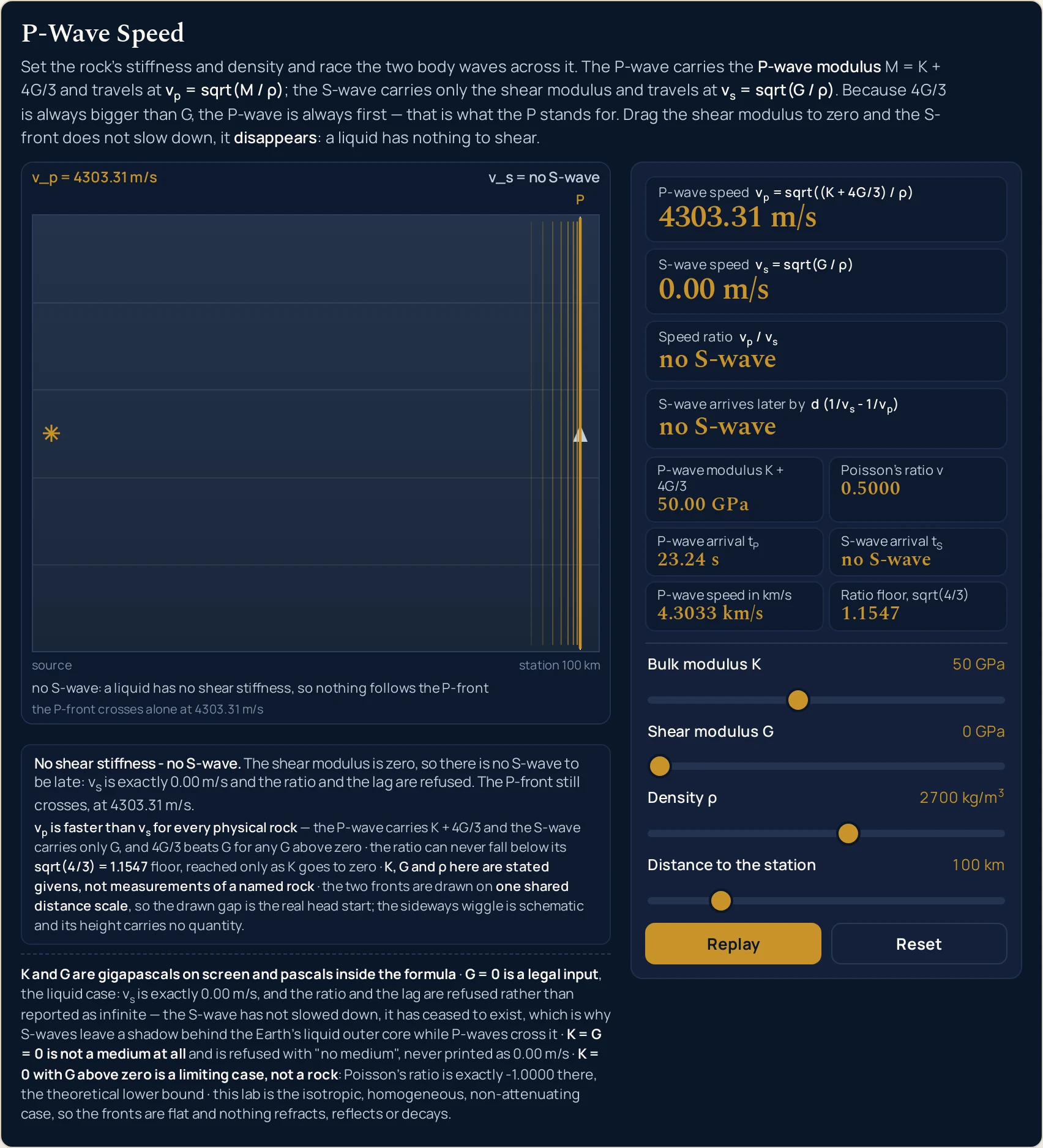
0.00 m/s and the ratio and lag cards read no S-wave, not an infinity. The P-wave card merely falls to 4303.31 m/s, and Poisson’s ratio is exactly 0.5000.Where the p-wave speed simulator breaks down
Every state the four sliders reach is answered, and the arithmetic is not where this panel can let you down. What it cannot be is a real path through real ground, and what it refuses to do is treat its own idealisations as facts. The first two items below matter more than the rest together.
- One uniform block, so the fronts stay flat
- This is the hard limit, and the panel states it in a standing line rather than hiding it. The lab draws the isotropic, homogeneous, non-attenuating case: one material from source to station, the same in every direction, losing nothing on the way. Real ground is layered, cracked, fluid-filled and faster along the bedding than across it, so nothing in this scene refracts, reflects, splits or fades. A speed measured over a real path is an average over all of that; this is the speed of a material.
- The sideways wiggle carries no quantity
- It is there to show that the S-front’s motion is across the path rather than along it, and nothing more. Its height is a drawing decision: there is no amplitude slider, no amplitude card and nothing on the panel that reports one, and the lab says so under the scene. Measure the wiggle and you have measured the renderer. The only distances in the picture that mean anything run along the path, where the two fronts share one scale.
- The resting picture is one instant, not the whole race
- The scene stops at the moment the P-front arrives, because that is when the head start is widest and most legible. It is not a claim that the S-front stops there: the lag card tells you how much further it has to go, and Replay runs the race again if you want to watch the gap open. A still of this lab is a snapshot of a chosen instant, chosen so that the gap is visible in every screenshot and every embedded view.
- Two of the four cases are not materials
- A bulk modulus of zero makes Poisson’s ratio exactly
-1.0000, the theoretical lower bound, and both moduli at zero is not a medium at all. The sliders reach those positions on purpose, to show where the bound is, and the caption strip names each one as a limiting case rather than letting it pass as a rock. Poisson’s ratio also goes negative well before that corner: atK = 50withG = 80 GPait reads-0.0217. - No frequency, no wavelength, no amplitude
- There is no frequency control on this panel, so the relation between a speed, a frequency and a wavelength is not something it can show you — the wave speed calculator and the guide to wavelength formulas and units are where that relation belongs. Nothing here says how a pulse spreads, loses height or changes shape as it travels, because there is no attenuation in the model at all.
- It runs the clock forwards only
- The distance slider sets a distance and the lab reports the gap. It cannot take a gap you measured and give you back the distance, which is the way the problem usually arrives in practice, and no control on the panel inverts it. That inverse is set out in the guide to transverse and longitudinal waves; the forward direction, from the moduli to the gap, is what this lab is for.
- Four slider positions, and no measurement anywhere
- You set four controls and the lab reports what they imply. There is no box to type a measured speed into, no unit menu and no way to run either relation backwards, and the bulk modulus, the shear modulus and the density are stated givens chosen to be legible — never properties attributed to a named rock. Verify any figure against your own source before you use it.
Where P-wave speeds are actually used
- Watching the head start grow with the distance
- This is what the fourth slider exists for, and it is the thing the calculator cannot show. Drag Distance to the station from end to end and the lag card runs from
1.27 sto63.40 swhile both speed cards sit perfectly still. The gap is bought at a fixed rate per kilometre, and the drawing redraws it to scale at every step, so the linear relationship is on screen rather than asserted. - Telling a liquid apart from a broken calculation
- A speed ratio that comes back as an infinity, a NaN or an enormous number is the commonest way this topic goes wrong, and the Melted preset is the state that produces it. Here the ratio card refuses instead, in words, while the S-wave card prints an exact
0.00 m/s. Stop one step short of that slider position and nothing breaks:1 GPaof shear stiffness gives a perfectly ordinary608.58 m/sand a ratio of7.1647. - Putting a floor under a ratio someone has handed you
- Any speed ratio below
1.1547is wrong before you check the arithmetic behind it, whatever the material, and that is exactly what the fixed grid cell is for. Load Ratio floor and the card above it lands on the cell, so the bound is demonstrated rather than quoted. The same check works upwards: a ratio of 4 or 5 means a very low shear modulus, which the sweep table above will place for you in one glance. - Seeing where the square root of 3 comes from
- The Crustal rock preset reads
1.7321, and the cell beside it reads0.2500. Those two numbers are not independent: Poisson’s ratio fixes the speed ratio on its own, and exactly a quarter is what produces sqrt(3). Move the shear slider one notch and both change together, which is the quickest way to see that the sqrt(3) is a condition rather than a fact about rock. - Comparing with the inside of the Earth, honestly
- The P-wave speed in km/s cell exists so the panel can be read against published figures, which are quoted that way rather than in m/s. It opens at
5.7735 km/s, and the ceiling is worth knowing before you try to match something: at the opening density of2700 kg/m3, both moduli at their maximum reach only9.1625 km/s. Going faster than that needs the density slider down as well —15.0555 km/sat1000 kg/m3— which is the panel making the point that a faster material is a different material. - Checking an arrival time you have worked out by hand
- The two arrival cells are the distance divided by each speed, and having both on screen with the lag card is enough to catch a dropped factor of a thousand straight away. At the opening rock they read
17.32 sand30.00 sover100 km. A kilometre read as a metre, or a km/s figure read as m/s, puts one of the three out by three orders of magnitude and the mismatch is immediate. - Separating the gentle first arrival from the damaging one
- The lab draws the P-front as a compression and the S-front behind it as a sideways motion, which is the whole reason the first arrival is the quieter one. It reports no amplitude and makes no claim about damage; the amplitude guide is where that side of the story belongs, and the speed of sound simulator is the contrasting case, a medium with no shear stiffness at all and therefore only one front.
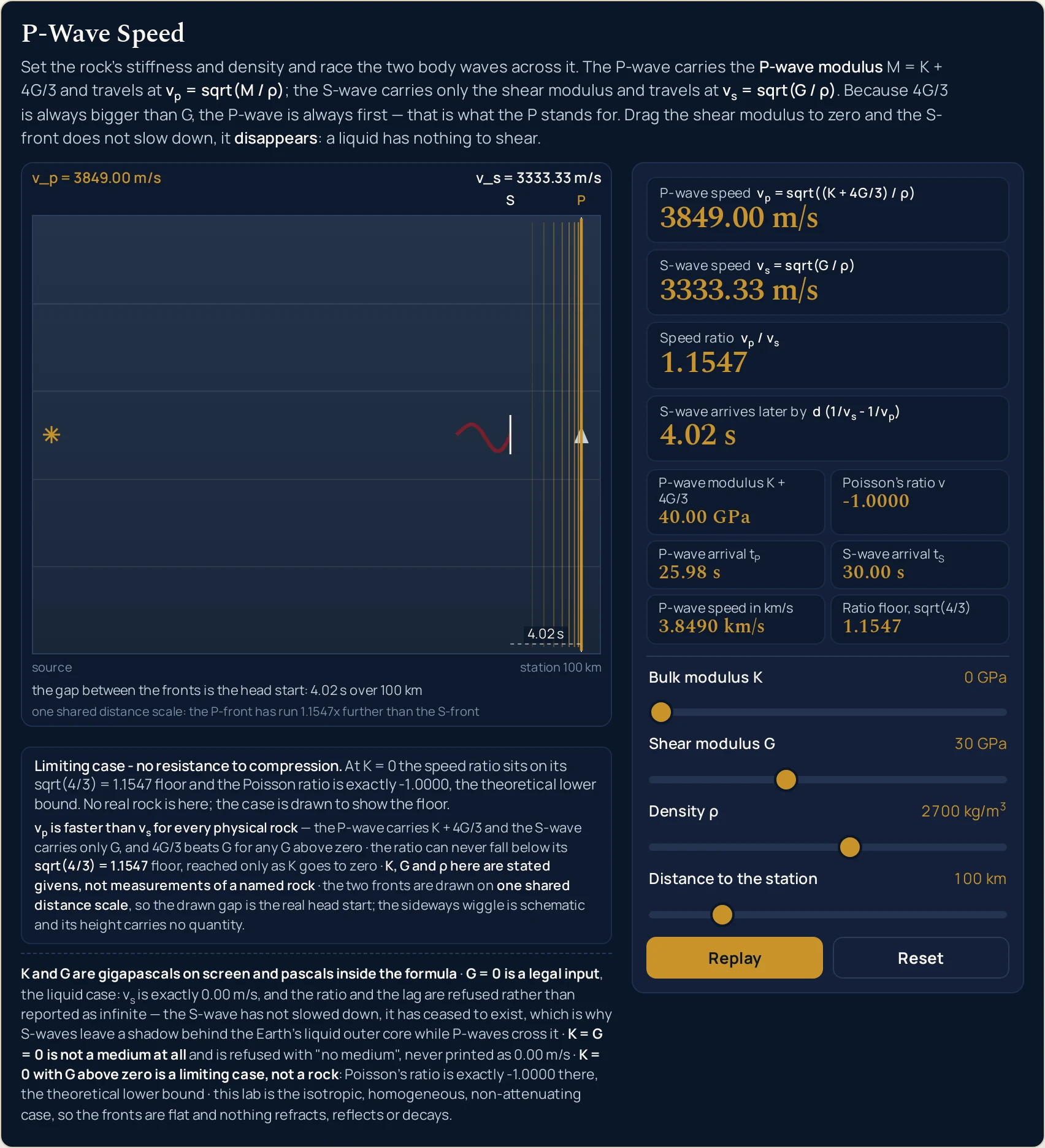
1.1547 — exactly the fixed floor cell under it — the two fronts come in 4.02 s apart, and Poisson’s ratio reads an exact -1.0000, the theoretical lower bound. The caption strip names it as a limiting case rather than letting it pass as a material.Where to go next
A panel can put you in a state and let you move one thing at a time, and that is the end of what a panel is for. The P-wave guide is where the subject is written out: the definition, the shear term argued from scratch, the fluid case, the measured velocities and eight problems with every step shown.
Three posts own the pieces this lab takes as read. The guide to transverse and longitudinal waves covers what separates the two body waves and how a distance comes out of their arrival gap, the guide to how sound waves travel covers the fluid case this relation reduces to when the shear modulus is zero, and the guide to wave speed in different media is the stiffness-against-inertia framing all of them share. The polar moment of inertia guide is where the shear modulus is a subject in its own right.
On the tool side, the P-wave speed calculator takes typed figures and solves in four directions, the speed of sound calculator handles the gas case, the wave speed calculator relates a speed to a frequency and a wavelength, and the Young's modulus calculator measures the third elastic modulus.
Two neighbouring pictures sit beside this one: the wave speed simulator and the speed of sound simulator. Beyond them there is the simulation library, an index of calculators, and the blog for everything written out at length.
Frequently asked questions
Why does the picture stop before the S-front reaches the station?
Because that is the instant the head start is largest and easiest to see. The race rests at the moment the P-front arrives, with the S-front still short of the station by the lag, and the dashed gap between the two is labelled with it: 12.68 s behind at the opening settings. Running on to the S-wave would park both fronts together and hide the whole point.
What does no S-wave on the ratio card mean?
It means the shear modulus is zero, so there is no S-wave for the ratio to be a ratio of. The S-wave speed card prints an exact 0.00 m/s, the ratio and the lag cards both print no S-wave, and the P-wave card still prints a number: 4303.31 m/s at a bulk modulus of 50 GPa and a density of 2700 kg/m³. An infinity would be the wrong answer rather than a bigger one.
Why does one zero print 0.00 and another print no medium?
Because they are different claims about the rock. With the shear modulus at zero and the bulk modulus above it there is still a medium, and an S-wave speed of exactly 0.00 m/s is the honest reading. With both moduli at zero there is nothing to carry a wave, so every speed-derived card prints no medium instead; the P-wave modulus cell still prints 0.00 GPa, which is what makes that refusal legible.
Does the sideways wiggle on the S-front show its amplitude?
No, and the lab states as much under the drawing: the wiggle is schematic and its height carries no quantity. The only distances in the picture that mean anything run along the path. Both fronts are drawn on one shared scale, so when the ratio card reads 1.7321 the P-front really is 1.7321 times further from the source than the S-front. Nothing on this panel reports an amplitude.
Why is the speed ratio exactly 1.7321 at the opening settings?
Because those three figures make Poisson ratio exactly 0.2500, and that one number fixes the ratio on its own. The stat grid prints it beside the ratio card so the two can be read together. Move the shear modulus and both change: at 20 GPa the ratio is 1.9579 and Poisson ratio 0.3235. The sqrt(3) is a consequence of that particular Poisson ratio, not a property of rock.
What is the ratio floor cell for, when it never changes?
It is a bound rather than a reading, so it holds at 1.1547 in every state, no medium included. That value is sqrt(4/3), the lowest the speed ratio can reach however compressible you make the rock, and it sits in the grid so the card above it can be checked against something fixed. Drag the bulk modulus to zero and the ratio card lands exactly on it.
Why do the two speeds not move when I drag the distance slider?
Because a distance is not in either speed formula. That slider moves only the clock: the two arrival cells, the lag card and the station label in the drawing. At the opening rock the lag runs 1.27 s over 10 km, 12.68 s over 100 km and 63.40 s over 500 km, exactly in proportion, while the two speed cards hold at 5773.50 and 3333.33 m/s throughout.
Why does this lab print 5773.50 m/s where the calculator prints 5773.5?
They are the same figure to different precision, and both are deliberate. Every speed card here carries two decimals, so the trailing zero is kept; the calculator drops trailing zeros in its headline and shows 5773.5, while its own chips use this two-decimal form. Neither is a measurement. Both are arithmetic on figures you set, so verify any value against your own source before you use it.
How many of the printed digits should I trust?
The two speeds and the three times carry two decimals, the ratio and Poisson ratio carry four, and the sliders are whole units apart from the density, which steps in fifties. Those are display choices rather than claims about accuracy. The lab measures nothing: the three material properties are stated givens, never properties of a named rock, and every digit is arithmetic on four slider positions.
References & formula source
- Every figure on this page comes from two relations and four slider positions. The P-wave speed is the square root of the P-wave modulus divided by the density, where the P-wave modulus is the bulk modulus plus four thirds of the shear modulus. The S-wave speed is the square root of the shear modulus divided by the density, which is a separate relation rather than a mode of the first. The panel applies both and multiplies out; the written guide derives them and works the problems.
- The three material properties are stated givens on every surface of this page and are never attributed to a named rock. We have no source for the density or either modulus of any real material, so inventing one would be worse than leaving it out. The only measured material figures quoted anywhere in this cluster are P-wave velocities, and they are in the reference at the foot of this list.
- A shear modulus of zero is a legal, meaningful setting rather than an error, and that is the single most important sentence in this list. The S-wave does not slow down as the rock melts; it ceases to exist. So the S-wave card prints an exact 0.00 m/s, the ratio and the lag refuse rather than reporting an infinity, and the P-wave speed merely falls, from 5773.50 to 4303.31 m/s at a bulk modulus of 50 GPa and a density of 2700 kg/m³.
- Two zero moduli are refused outright, and for a different reason. With both sliders at the bottom there is no medium at all, so a speed of 0.00 m/s would claim a wave that arrives after infinite time; every speed-derived card prints no medium instead. The P-wave modulus cell still prints 0.00 GPa, because that modulus really is zero and saying so is what makes the refusal legible. The ratio floor cell still prints 1.1547, because a mathematical bound is not a state of the rock.
- The moduli are gigapascals on the sliders and pascals inside the formula, a factor of 1e9 the lab applies for you. By hand that is the step most often skipped, and skipping it is a factor of a thousand million. Speeds are metres per second on every card; the kilometres-per-second cell is a convenience for comparing with the geophysical literature, which quotes P-wave speeds that way, and it is always on screen beside the metres-per-second figure so the two cannot drift apart.
- The drawing states its own scale rules rather than leaving them to be assumed. The two fronts share one distance scale, so the drawn gap between them is the real head start and the drawn ratio of their distances is the computed speed ratio. The picture comes to rest at the moment the P-front arrives, which is the state that makes that gap visible. The sideways wiggle on the S-front is schematic: its height carries no quantity, and nothing on the panel reports an amplitude.
- The relation drawn here is the isotropic, homogeneous, non-attenuating case and nothing more. Real ground is layered, cracked, fluid-filled and faster along the bedding than across it, so a speed measured over a real path is an average over all of that. The lab has no frequency, no wavelength and no amplitude, nothing refracts, reflects or decays in it, and it computes no distance from a gap between two arrivals. It gives the speed of a material, never of a structure.
- The simulation was built, gated and frozen before this page was written, and every string quoted here was read back out of the running file rather than computed here. A reference oracle at 156 checks with none failing; a Node tier at 440 checks with none failing; a headless Chrome tier at 1233 checks with none failing; a mutation pass over 118 planted faults with 110 killed, eight proven redundant by executed double and triple mutants, and no unexplained survivors; a compact-height pass measured at 918 pixels against a 1000 pixel ceiling; and a cross-browser pass of 19 checks in which all 114 readouts came out identical in Chrome and in Firefox at each of four widths.
- What was not verified, stated as a gap rather than left to be assumed. Safari and WebKit: the build on the machine this was tested on cannot start, so Safari was never exercised and nothing here is evidence about it. Assistive technology: every slider carries a label and a spoken value and the drawing carries a full description, but no screen reader was driven and no real touch target was pressed. No figure on this page has been checked against a physical measurement of any kind.
- Nothing on this page is a measurement. Every digit and every pixel is arithmetic on four slider positions, so the lab shows the shape of two relations rather than an observation of any rock, and the model is one uniform block between one source and one station. Verify any figure against your own source before you use it for anything that matters.
- Further reading: P-wave — Wikipedia