The magnetic flux simulator is a free interactive lab for the one quantity a field strength cannot give you on its own: how much of that field a tilted surface actually catches. Set a flux density in millitesla, a loop area in square centimetres and an angle from the normal in degrees; the four cards report the flux, the facing area, the angle factor and a drawn line count, and the canvas narrows the loop’s shaded face to match. Hold the first two sliders still and the tilt alone carries the flux card from 1.000 mWb through 0.000 mWb to -1.000 mWb. Nothing on the panel is time-derived, so no voltage is calculated anywhere in it.
Magnetic Flux
A loop tilting in a uniform field. Magnetic flux is how much field gets through a surface: Φ = B A cos θ, where θ is the angle between the field and the loop's normal — the line sticking out at right angles to its face, never the face itself. Hold the flux density and the area still and drag the angle: the flux falls to zero edge-on at 90° and comes back with the opposite sense past it. Nothing here changes with time, so no voltage is calculated anywhere.
Load a real case onto the simulator
Each button stops the sweep, restores the three sliders and then writes its own values, so a load never inherits half of the previous case or walks off its own angle. The status line underneath quotes the panel straight back rather than storing any text of its own. The first four hold the field and the loop still and move only the tilt; the fifth changes both the other sliders and lands on a flux you have already seen.
Pick a case above, or drag the three sliders yourself.
What Is the Magnetic Flux Simulator?
The magnetic flux simulator is a free interactive physics lab that runs in your browser, with nothing to install and no sign-up. It is built around one relation, Φ = B A cos θ, and around the one thing about it that is hard to credit on paper: the field can stay exactly as it is while the reading falls to nothing and comes back the other way. Three sliders set the flux density, the loop area and the angle from the normal; four cards answer, and a drawing underneath shows the loop as the field sees it.
The angle is measured from the normal to the loop — the line sticking out at right angles to its face — and never from the face itself. At the boot setting the loop is square to the field and the cards read Magnetic flux 1.000 mWb, Area facing the field 50.00 cm2, Angle factor 1.000 and Field lines through the loop 5. Drag the angle to 60 degrees and they read 0.500 mWb, 25.00 cm2, 0.500 and 3, with nothing else touched.
Two settings are the whole point of the lab. Edge-on at 90 degrees the field skims past the face: 0.000 mWb, 0.00 cm2, 0.000, no lines drawn at all, and Which way it threads reads none. Carry the same slider on to 180 degrees and the loop has been turned right over: -1.000 mWb at an angle factor of -1.000, the same size of flux with the opposite sense, and Which way it threads reads into the loop. The sign records which way the flux threads the normal you chose, not a side the field itself prefers.
A compact grid under the cards keeps the quantities a reader has to compare. It prints the flux density in tesla, 0.200 T, beside the loop area in square metres, 0.0050 m2, the most that field and that loop could ever give, the flux in webers as 1.000e-3 Wb, the angle as 0 deg from the normal and the sense as out of the loop. A flux density is a field at a point and a flux is a total through a surface, and seeing a tesla and a weber on one screen is the fastest way to stop treating them as one quantity.
Two honesty notes belong on the drawing rather than in the small print. The gold lines through the loop stand for 0.2 mWb of flux each, so the count is a counting aid and not a physical tally of anything. And nothing in this lab changes with time, so no voltage is calculated anywhere in it: the Rotate button is a way of sweeping the angle without dragging, not a demonstration of a changing flux.
| Control | Range and step | What moves when you use it |
|---|---|---|
| Flux density B | 0 to 500 mT, step 10 mT | Boots at 200 mT. Scales the flux and the drawn line count in proportion, and never moves the angle factor: at 0 mT the flux reads 0.000 mWb while the angle factor still reads 1.000. |
| Loop area A | 1 to 100 cm2, step 1 cm2 | Boots at 50 cm2. Scales the flux and the area facing the field together, in the same proportion, and leaves the angle factor alone. |
| Angle from the normal | 0 to 180 deg, step 5 deg | Boots at 0 deg. The only control that can take the flux to zero or reverse its sense: 90 deg gives 0.000 mWb, and 180 deg gives -1.000 mWb at the boot field and area. |
| Rotate / Pause | button, boots paused | Sweeps the angle 0 up to 180 and back at about 30 deg/s, snapped to the 5-degree slider grid so every reading is one you can also dial in by hand. The label toggles. |
| Reset | button | Puts all three sliders back to 200 mT, 50 cm2 and 0 deg and stops the rotation. It is the only control that touches more than one thing at once. |
How to use the magnetic flux simulator
- Read the four cards before you touch a control. The lab boots paused and square on, so Magnetic flux reads
1.000 mWb, Area facing the field50.00 cm2, Angle factor1.000and Field lines through the loop5. Each card carries the thing that produced it in its own label, so the headline is labelledΦ = B A cos θand the second cardA cos θ, size only. - Leave Flux density B at
200 mTand Loop area A at50 cm2, and drag Angle from the normal to60 deg. The flux halves to0.500 mWb, the facing area halves to25.00 cm2, the angle factor is0.500and two of the five gold lines go, leaving3. Nothing about the field moved; the grid cell still reads0.200 T. - Carry the same slider on to
90 deg. This is the step the lab exists for. Magnetic flux reaches0.000 mWbwhile Area facing the field reaches0.00 cm2, the angle factor is0.000, no lines are drawn at all, and Which way it threads readsnone. The field is as strong as it ever was and the loop is the same loop. - Keep going to
180 deg. The flux comes back as-1.000 mWb, the facing area returns to the full50.00 cm2, the angle factor is-1.000and the five lines are drawn again. Which way it threads now readsinto the loop: the same size of flux through the same area, arriving at the other face. - Now drag Flux density B instead, and watch what refuses to move. At
0 mTthe flux reads0.000 mWband no lines are drawn, but Angle factor still reads1.000, because the cosine is a fact about the geometry and knows nothing about the field. Take the slider to500 mTand the flux is2.500 mWbat13lines, with the facing area unchanged at50.00 cm2. - Drag Loop area A and the flux follows it in exactly the same proportion. At
100 cm2the flux is2.000 mWband the facing area100.00 cm2; at1 cm2they are0.020 mWband1.00 cm2. Flux is linear in the field and linear in the area, and these two steps are that statement with the numbers attached. - Press
Rotatewhen you would rather watch than drag. The label turns toPauseand the angle sweeps 0 up to 180 and back at about 30 deg/s, snapped to the same 5-degree grid the slider uses, so every reading that flashes past is one you can also hold still. The dot on the lower plot runs along the cosine curve, through the zero crossing and down to the bottom. - Press
Resetwhenever you have lost your place. It returns all three sliders to200 mT,50 cm2and0 degand stops the sweep, which is why every preset button above presses it first. It is the only control that reaches more than one thing at a time. - Read the compact grid last, because it is the part that settles arguments. Most it could be gives the flux this field and this loop would carry square on, so you can see at a glance what the tilt has cost; Flux in webers repeats the headline in SI units as
1.000e-3 Wb; and Angle prints0 deg from the normalwith the line it is measured from named in the value itself. - Read the caption under the drawing as a claim about the drawing. Square on it says
loop square to the field - maximum flux; edge-on,edge-on - no flux threads the loop; past 90 degrees,flipped past 90 deg - the flux reverses. Under it sitseach line drawn through the loop is 0.2 mWb, and the gold lines really are drawn in the number the card reports.
The step worth repeating is the third one. Load Loop square to the field, then drag the tilt to 90 deg with your eye on the grid rather than on the headline. 0.200 T does not budge while 1.000 mWb becomes 0.000 mWb, and that is the whole difference between a flux and a flux density on one screen. If you want typed figures rather than the 5-degree grid — 35.5 deg, say, or a field well past this slider’s top end — the magnetic flux calculator takes the same three quantities as boxes and prints the substitution.
For what a flux is — the definition, the weber written three ways, the full geometry in prose, why the net flux out of a closed surface is zero and seven worked problems — read the magnetic flux guide. This page is about the panel and the drawing: which card answers which question, which slider can and cannot move each of them, and where the picture gives up before the numbers do.
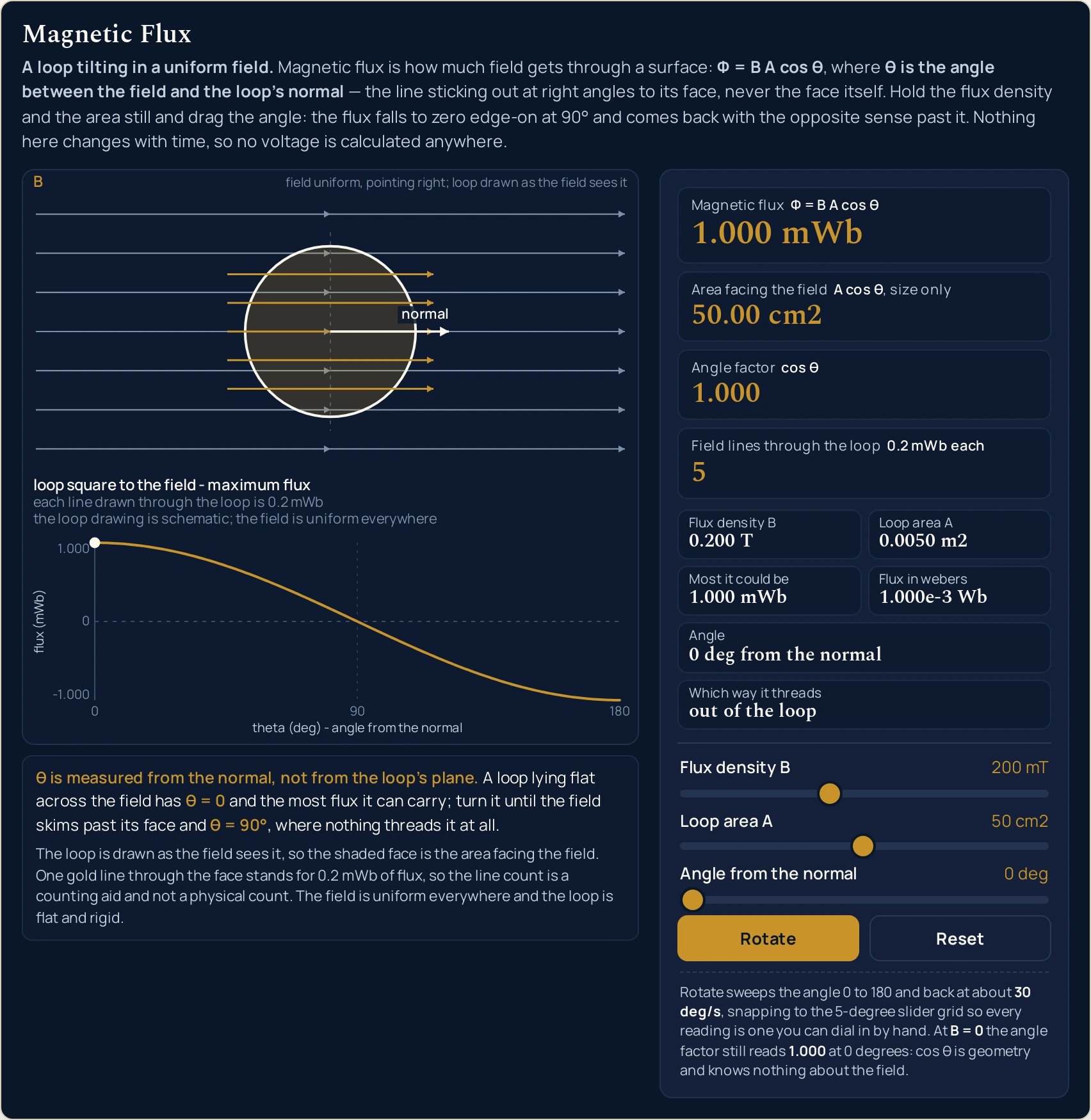
200 mT through 50 cm2 with the loop square to the field. Magnetic flux reads 1.000 mWb, Area facing the field the whole 50.00 cm2, Angle factor 1.000 and Field lines through the loop 5. There is no angle arc on the drawing, because at 0 deg there is no angle to mark.Worked example: change one thing at a time
Every row below is one setting of the three sliders, and every cell is a string the running lab printed there. The first four hold the field and the loop still and move only the tilt; the fifth changes both of the other two. If one of these cells and the running panel ever disagree, the panel is the one to trust.
| Flux density | Loop area | Angle from the normal | Angle factor | Area facing the field | Flux |
|---|---|---|---|---|---|
| 200 mT | 50 cm2 | 0 deg | 1.000 | 50.00 cm2 | 1.000 mWb |
| 200 mT | 50 cm2 | 60 deg | 0.500 | 25.00 cm2 | 0.500 mWb |
| 200 mT | 50 cm2 | 90 deg | 0.000 | 0.00 cm2 | 0.000 mWb |
| 200 mT | 50 cm2 | 180 deg | -1.000 | 50.00 cm2 | -1.000 mWb |
| 500 mT | 10 cm2 | 0 deg | 1.000 | 10.00 cm2 | 0.500 mWb |
Rows 1 to 3 are the argument of the page in three lines. The first two columns never change, so whatever happens to the last column is the tilt’s doing and nothing else’s. The angle factor and the facing area fall together, in step, from 1.000 and 50.00 cm2 through 0.500 and 25.00 cm2 to 0.000 and 0.00 cm2.
Row 4 is the one that surprises people. At 180 deg the facing area is back at 50.00 cm2 — the full area, exactly as in row 1 — while the flux reads -1.000 mWb. That is deliberate: the facing-area card reports a size, so it cannot tell you which face is doing the facing, and the sign is carried by the flux card and by the sense cell instead.
Rows 2 and 5 are the pair to read against each other. Both print 0.500 mWb, and they get there by routes that have nothing in common: row 2 by halving a full loop with a tilt, row 5 by putting a fifth of the area into a field two and a half times as strong, square on. Their angle factors are 0.500 and 1.000, and Most it could be separates them outright at 1.000 mWb against 0.500 mWb. A flux reading alone cannot say which of the two you are looking at.
One pair in this table does not mean what it looks like. Take Flux density B to 0 mT with the loop square on and the flux reads 0.000 mWb while the angle factor reads 1.000 — the same angle-factor cell as row 1, beside the same flux cell as row 3. Neither follows from the other: the factor is the cosine of the tilt and the flux is the product of all three quantities, and a field of zero takes the product to nothing without touching the geometry. The field itself is what the guide to the magnetic field covers.
Formula and symbol reference
The panel prints the relation inside the label of the card it feeds, so an answer never arrives without the rule: Φ = B A cos θ sits above Magnetic flux, A cos θ, size only above the facing area and cos θ above the angle factor. There is no physical constant anywhere in it, which means every figure the lab reports is exact arithmetic on three slider values.
The last column below is each slider’s own end stops rather than the range the physics allows, and that distinction matters when a real field runs off the end of one. The field slider stops at 500 mT, which is half a tesla, so any field stronger than that has to go to the magnetic flux calculator, whose field box takes tesla directly and has no top end. For the field a long winding produces in the first place, the solenoid magnetic field calculator solves B = µ0 n I for any one of its three quantities — it has no area and no angle, so its answer is the number you then bring to this panel.
| Symbol | Meaning | SI unit | In this lab |
|---|---|---|---|
| Φ | Magnetic flux: the whole point of the lab, and the only quantity on the panel that can be negative. The headline card prints the relation that produced it, so the answer never arrives without the rule | weber (Wb) | Three decimals of a milliweber on the card and a four-figure mantissa in the grid. Across both sliders it runs 0.000 mWb to 5.000 mWb and down to -5.000 mWb; the grid writes the boot reading as 1.000e-3 Wb. |
| B | Magnetic flux density: the field at a point, and the thing a tesla measures. The slider is in millitesla because that is the band school problems live in; the grid repeats it in tesla | tesla (T) | 0 mT to 500 mT in steps of 10 mT, printed beside the slider as 200 mT at the boot value. The grid shows the same field as 0.200 T, and 0.000 T or 0.500 T at the slider ends. |
| A | Loop area: the loop’s own area, not the part of it facing the field. Any flat shape of that area behaves identically here, because the relation asks the surface for nothing else | square metre | 1 cm2 to 100 cm2 in steps of 1 cm2, printed as 50 cm2 at the boot value. In the grid that is 0.0050 m2, with 0.0001 m2 and 0.0100 m2 at the ends. |
| θ | Angle from the normal: the angle between the field and the line at right angles to the loop’s face. The whole page turns on where it is measured from, which is why the grid cell spells the line out in its own value | degree (the SI unit is the radian) | 0 deg to 180 deg in steps of 5 deg, printed as 0 deg at the boot value. The grid reads 0 deg from the normal, 90 deg from the normal or 180 deg from the normal. |
| A cos θ | Area facing the field: the shadow the loop casts across the field, and the only part of it the flux counts. The card reports its size, so it never goes negative | square metre | A working value, never an input. 50.00 cm2 square on, 25.00 cm2 at both 60 and 120 degrees, 0.00 cm2 edge-on, and 50.00 cm2 again flipped right over. |
| cos θ | Angle factor: the fraction of the full flux that survives the tilt. It is a fact about the geometry alone and does not know what the field is doing | dimensionless | Signed, to three decimals: 1.000 at 0 degrees, 0.866 at 30, 0.707 at 45, 0.500 at 60, 0.000 at 90 and -1.000 at 180. It still reads 1.000 with the field slider at zero. |
| B A | Most it could be: the flux this field through this loop would give with the loop square on. It is a product, so it has no denominator and divides nothing | weber (Wb) | 1.000 mWb at the boot field and area, 0.500 mWb for the stronger field through the smaller loop, 5.000 mWb at the top of both sliders and 0.000 mWb with the field at zero. |
| lines drawn | Field lines through the loop: the flux divided into equal drawn parts and rounded to a whole number of them, so a reading can be counted rather than read | a count, at 0.2 mWb a line | An integer from 0 to 25: 5 at the boot setting, 3 at 60 degrees, 0 edge-on, 5 again flipped right over, and 25 at the top of both sliders. |
The compact grid under the four cards is there to hold the quantities a reader has to compare, in the order the build settled on: the four numeric cells first, then the two whose values are sentences and therefore get a full-width row each rather than being cut off halfway through their own claim.
| Cell | What it is for | Square on | Edge-on | Flipped right over |
|---|---|---|---|---|
| Flux density B | the field itself, in tesla rather than the slider’s millitesla | 0.200 T |
0.200 T |
0.200 T |
| Loop area A | the loop’s true area in SI units, which is what the relation wants | 0.0050 m2 |
0.0050 m2 |
0.0050 m2 |
| Most it could be | the product of those two — the flux this field and this loop would give square on, and the ceiling every other reading sits under | 1.000 mWb |
1.000 mWb |
1.000 mWb |
| Flux in webers | the headline card again in SI units, so a milliweber never has to be converted by hand | 1.000e-3 Wb |
0.000e+0 Wb |
-1.000e-3 Wb |
| Angle | the tilt, with the line it is measured from named in the value itself | 0 deg from the normal |
90 deg from the normal |
180 deg from the normal |
| Which way it threads | the sense, in words rather than as a sign | out of the loop |
none |
into the loop |
Two of those cells are worth a warning. Most it could be is a product and divides nothing at all, so it is immune to every edge the rest of the panel has to guard against; and Flux in webers prints 0.000e+0 Wb at zero, with one exponent digit and no sign, because the flux card never prints a negative zero.
The physics: why the drawing narrows and the field does not
The upper band of the drawing is not a side view and not a plan view. The loop is drawn as the field sees it — looking straight along B — and the note in the corner of the canvas says so in as many words: field uniform, pointing right; loop drawn as the field sees it.
That one choice is what makes the shading mean anything. In that view the shaded face narrows in exactly the ratio the facing area falls by, so the width you can see is the quantity the second card reports. Drawn in perspective the shading would be decoration, and the narrowing to a bare vertical line at 90 degrees would look like an accident of the angle rather than the point of the lab.
The field arrows are the other half of the argument, and they never change. They stay evenly spaced, the same length and pointing the same way whatever the three sliders are doing, because a uniform field is the model. Every one of those arrows is still crossing the space the loop sits in when the flux card reads 0.000 mWb; what has gone is not the field but the opening presented to it.
The dashed vertical line through the middle of the loop is the axis it pivots about, and it is drawn so the turning is readable as a rotation rather than as the loop shrinking. The short arrow out of the centre labelled normal is the line the angle is measured from, and the arc labelled theta appears between it and the field at every setting but 0 deg, where there is no angle to mark.
The lower band plots the flux against the tilt over the whole 0 to 180 range, with a zero line and a filled dot at the current angle. Its two end ticks are not fixed: they are Most it could be and its negative, so they read 1.000 and -1.000 at the boot setting and 0.500 and -0.500 for the stronger field through the smaller loop. With the field slider at zero there is nothing to scale by and the plot prints no end ticks at all, with the dot sitting on the zero line.
Its horizontal axis is titled theta (deg) - angle from the normal where there is room for it, and simply theta (deg) where there is not, which on a phone is what you get. Spending the slack on naming the line the angle comes from is deliberate: it is the single thing this topic goes wrong on, and the axis of the graph is the last place a reader looks before they believe the shape of the curve.
The curve itself is the best argument on the page that the cosine is not a fudge factor. It is flat near 0 degrees, so the first few notches of tilt cost almost nothing — the angle factor is still 0.996 at 5 deg and 0.966 at 15 deg. It is steepest at the zero crossing, where five degrees either side of edge-on is the difference between 0.087 and -0.087. A sensor a few degrees out of alignment barely notices; one near edge-on notices everything.
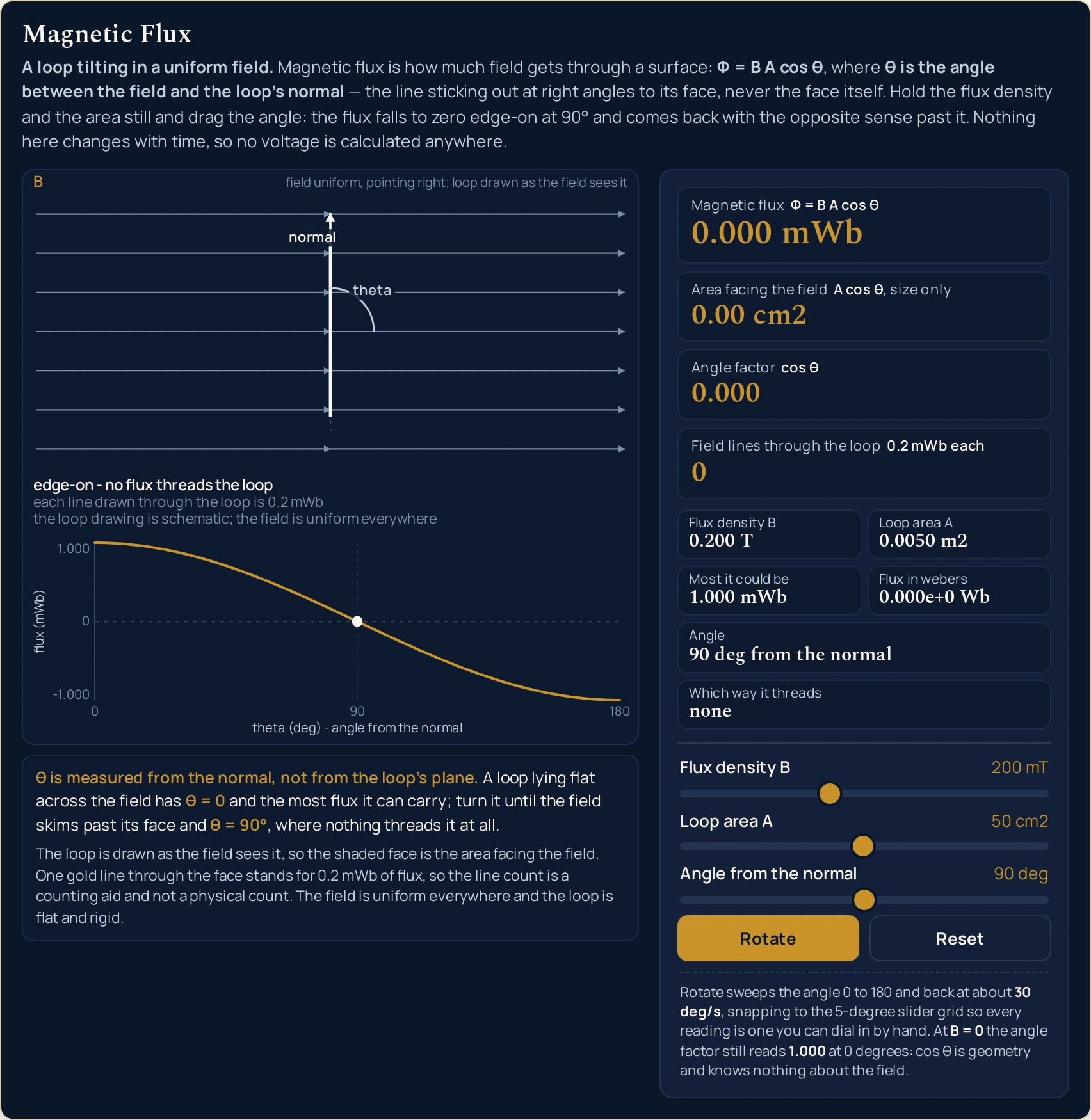
0.000 mWb, Area facing the field 0.00 cm2, Angle factor 0.000 and Field lines through the loop 0, while Flux density B is unchanged at 0.200 T. The shaded face has narrowed to a vertical line and the dot on the plot sits on the zero crossing.Where the magnetic flux simulator breaks down
The lab solves its own model exactly, so nothing on the screen ever fails. Everything below is a limit of that model, of the grids the three sliders move on, or of what a canvas a few hundred pixels wide can honestly carry.
- The field is uniform everywhere and never runs out
- Watch the arrows while you drag any of the three sliders: they keep the same length, the same spacing and the same direction right across the band, and nothing the loop does disturbs one of them. That is the model stated on the canvas, and it is a fair one inside a long winding or across a small patch of a large magnet.
- It is a poor one for a wide loop held close to a small magnet, where the field at the loop’s rim is weaker than at its centre and leaning a different way as well — and a single Flux density B slider has no way of saying so. The panel will hand you a figure regardless; what it cannot do is warn you that one number was never going to be enough.
- The loop is flat and rigid, so it has exactly one normal
- There is one angle slider, so there is one normal arrow on the drawing, and that is only honest for a surface whose face points the same way all over. Bend or fold it and the arrow would have to be drawn in a different direction at every point of the rim, with its own share of the flux counted separately — no setting of these three sliders can reach that. The loop never deforms either: dragging Loop area A grows and shrinks the circle on screen without ever creasing it.
- The drawn lines are a counting aid, not a count of anything
- Each gold line through the face stands for
0.2 mWb, and the card reports the flux divided by that and rounded to a whole number, which runs0to25across the slider box. Field lines are a drawing convention and not objects, so nothing is being tallied. What the count is good for is noticing a change you would otherwise have to read: three lines instead of five is a halving you can see from across a room. - Nothing changes with time, so no voltage is computed anywhere in this lab
- There is no time control, no rate of change and no EMF readout, and the
Rotatebutton is a convenience for sweeping the angle rather than a demonstration of a changing flux: it snaps to the slider grid precisely so that every frame is a setting you could have dialled in and held. A flux that genuinely changes drives an EMF round a circuit, which is Faraday’s law, and the Faraday's law formula guide owns that relation. The lab for it is the electromagnetic induction simulator, whose controls are a drive frequency, a turns count, a field and a coil area — and no angle at all, which is the gap this one fills. - The three sliders land on grids, and nothing between two notches is reachable
- The field moves in
10 mTsteps, the area in1 cm2steps and the angle in5 degsteps, which is coarse on purpose: every reading the lab shows is one you can get back to, and that includes every frame the sweep flashes past. It also means the readings here are a sample of the cosine rather than the whole of it. A tilt of35.5 deg, or any field past500 mT, belongs in a box rather than on a slider. - The facing-area card cannot tell you which face is facing
- It reports a size, so
50.00 cm2at0 degand50.00 cm2at180 degare the same reading for two opposite situations, and25.00 cm2appears at both60 degand120 deg. That is the honest choice — a card reading minus fifty square centimetres would raise a question about negative areas that has no good answer — but it does mean that card alone never settles a sense. Read the sign off the flux card and the words out of the sense cell. - The sign is a choice you are being shown, not a direction in space
- Out of the loop and into the loop are statements about the normal the lab has drawn, which is the one pointing out of the shaded face. Flip that choice and every sign the panel prints flips with it, without one thing about the field having changed. A worked answer that comes out the other way up has usually started from the other face, which is a disagreement about labelling and not about physics. Which way an induced current then runs is a different question again, and the Lenz's law guide is where it belongs.
- The canvas gives words up before it gives numbers up
- Narrow the window and the caption lines fall back through shorter forms in a fixed order, so
loop square to the field - maximum fluxbecomessquare to the field: maximum fluxand thenmaximum flux, while the axis title drops totheta (deg). A line that will not fit in any of its forms ends the strip rather than being skipped, so what survives is always a contiguous run from the top. The four cards never degrade at all, so a phone shows the full answer in the panel even where the drawing has given most of its labels away. - A coil of several turns is a different quantity, and this lab has no turns control
- Winding the wire round the same hole twice does not make more field pass through it, so the flux is unchanged; what changes is the quantity you get by multiplying it by the number of turns, which the Faraday's law formula guide calls the flux linkage. There is deliberately no turns slider here, because a flux belongs to the surface rather than to the wire. Take the figure off this panel and multiply it yourself if that is what your problem wants.
- Nothing here has been measured, and two of three engines were tested
- Three slider positions go in and one idealised figure comes out; a preset name is only a label for the values it writes. No magnet, core, coil or instrument is described anywhere on this page, and no measured field, geometry or material appears, because no source for one was fetched for this cluster. The readouts were compared in Chrome and Firefox and agreed at every width checked; the WebKit build on that machine could not be launched, so nothing here is claimed about Safari.
Where magnetic flux is actually used
- Setting a core’s working point on two sliders
- A transformer or motor designer carries two figures at once: the total flux the magnetic circuit has to pass, in webers, and how hard that flux is being pushed through each square metre of steel, in tesla, because past a certain density the iron saturates and stops helping. Those are the headline card and the Flux density B cell, and the Loop area A slider is the cross-section between them. No saturation figure is quoted on this page, because the density steel gives up at is a property of the particular material and its working conditions rather than of this relation — verify before use.
- Costing a sensor’s misalignment in one drag
- A flux-gate or search-coil sensor responds to the field along its own axis, so mounting it a few degrees off costs you the cosine of the error. Drag the angle one notch from square on and Angle factor reads
0.996; three notches,0.966. That is the practical form of a result the curve makes obvious: alignment is forgiving near square on and brutal near edge-on, where the same five degrees moves the factor from0.087to-0.087and takes the sense with it. - Sizing the flux through a small head or pickup
- A tape head, a stripe reader or a search coil is a small loop with a field through it, so its reading is set by the same three quantities and by nothing else. Take Loop area A down to
1 cm2and the lab is working in the band those devices live in: at200 mTsquare on the flux is0.020 mWb, which is twenty microwebers. The arithmetic is this panel’s; the figures for any particular device are not ours to quote — verify before use. - Settling the sign question in front of a class
- This is the fastest thing the lab does. Load Flipped right over and the flux is
-1.000 mWbwhile the facing area is the full50.00 cm2, with the sense cell readinginto the loopin words rather than leaving a minus sign to be interpreted. Then point out that the only thing making it negative is which face the drawn normal came out of, which is a choice and not a measurement. - Talking about a scanner magnet without pretending to measure one
- An MRI magnet is specified by its flux density, and the flux matters for everything that sits in it with a surface: a receiver coil, a screening panel, a steel trolley. The geometry is exactly this panel’s — a field, an area and an angle from the normal — but the field itself is past the top of this slider, so the lab can show you the shape of the answer and not the size of it. No figure for any particular scanner appears on this page, because none was sourced for it — verify before use.
- Auditing a flux you already have
- The commonest use of a panel like this is checking a figure rather than producing one. Any flux larger in size than Most it could be is wrong before the working is even read, because the angle factor can never exceed
1.000in either direction. Set the field and the area a problem gives you, read that cell, and compare: it is a one-line sanity check that catches an upside-down cosine and a square-centimetre area left unconverted. - Getting a genuinely uniform field to feed in
- The model assumes one, and the usual real source of one is the inside of a long winding, where the field is very nearly constant over the middle. The solenoid simulator is where that field comes from — it reports the field inside the coil and the flux through one of its turns, with no surface to tilt — and the figure it gives is the one to bring to the Flux density B slider here.
- Seeing why anyone wants the number at all
- A steady flux does nothing by itself, which is a fair question to raise about a panel that computes one. The answer is that a flux which changes drives a current round a circuit, and the electromagnetic induction guide covers that phenomenon end to end. What this lab is for is the ingredient: getting the geometry of the flux right before anything is allowed to change.
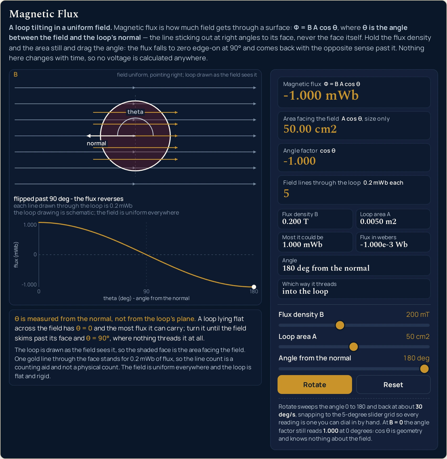
180 deg from the normal. Magnetic flux reads -1.000 mWb and Angle factor -1.000, while Area facing the field is back at the full 50.00 cm2 and five lines are drawn again. Which way it threads reads into the loop, and the dot on the plot sits at the bottom of the curve.Where to go next
The topic itself — what a flux is, what the weber measures, the geometry in prose, what happens past 90 degrees, why the net flux out of a closed surface is zero and seven problems end to end — is in Magnetic Flux: Formula, Units and Worked Examples. When you need figures the sliders cannot reach, the magnetic flux calculator takes any three of the flux, the flux density, the area and the angle and returns the fourth with the working.
The field side of the story has tools of its own. The guide to the magnetic field covers what a flux density is and where it comes from, the solenoid magnetic field calculator turns a turns density and a current into one, and the magnetic field and Lorentz force lab puts a moving charge into a uniform field instead of a surface. The guide to the solenoid with the solenoid lab is where a uniform field actually comes from, and the guide to electromagnets takes the same winding further.
Downstream of this page, the Faraday's law formula guide and the guide to electromagnetic induction pick the story up at a flux that changes, with the electromagnetic induction lab for the moving case; the Lenz's law guide and the Lenz law lab fix which way the result runs, and the guide to eddy currents is what happens when the conductor is a sheet rather than a loop. The rest is in the library of physics simulations.
Frequently asked questions
The panel prints a flux density in tesla and a flux in webers at the same time. Is that the same number twice?
No, and having both on one screen is the quickest cure for treating them as one quantity. Flux density B is the field at a point: the grid cell reads 0.200 T and stays there however far you tilt the loop. Flux is a total through the whole face: the headline card runs from 1.000 mWb down through 0.000 mWb and on to -1.000 mWb while that tesla figure does not move at all.
Why does the Angle from the normal slider read 0 degrees when the loop is facing the field?
Because the angle is measured from the loop’s normal, which is the line sticking out at right angles to its face, and that line points along the field when the loop faces it square on. The grid spells it out as 0 deg from the normal. Measure from the face instead and you have the complement, which puts a sine where the cosine belongs and turns a square-on loop into a 90-degree reading.
With Flux density B dragged to zero the Angle factor still reads 1.000 while the flux reads 0.000 mWb. Is one of them wrong?
Both are right, and the pair is worth a moment. The angle factor is the cosine of the angle and nothing else, so it is a fact about the geometry that knows nothing whatever about the field: at 0 degrees it is 1.000 whether the field is 500 mT or nothing at all. The flux is the product of all three, so a field of zero takes it to 0.000 mWb on its own.
Why does Area facing the field read 50.00 cm2 at 0 degrees and again at 180 degrees?
Because that card reports a size and never a signed value. Turning the loop right over presents the same area to the field as leaving it square on, so the facing area is identical at the two settings; what has changed is which face is doing the presenting. The sign lives on the headline card, which reads 1.000 mWb at 0 degrees and -1.000 mWb at 180, and in the sense cell.
What exactly do the gold lines through the loop count?
One drawn line stands for 0.2 mWb of flux, and the card prints how many the current reading comes to: 5 at the boot setting, 3 at 60 degrees, none at all edge-on, and 25 at the top of both sliders. It is a counting aid rather than a tally of anything physical — field lines are a drawing convention, not objects — but the canvas really does draw the number the card claims.
Does the Rotate button show me anything the Angle from the normal slider cannot?
No, and it is not meant to. It sweeps the angle from 0 up to 180 and back at about 30 degrees a second, snapping to the same 5-degree grid the slider uses, so every reading it flashes up is one you can also dial in by hand and hold still. Press it again and the label turns back to Rotate with the lab stopped wherever the sweep had got to.
Why is the loop drawn as a narrowing band rather than as a tilted rectangle in perspective?
Because the drawing shows the loop as the field sees it, looking straight along B, and the note in the corner of the canvas says so. That is the one view in which the shaded width is in the same ratio as the facing area, which is what makes the shading mean something. Drawn as a plan view the shading would be decoration, and the narrowing to a line edge-on would be a coincidence rather than the point.
Does Reset put the rotation back as well as the three sliders?
Yes, both. It returns Flux density B to 200 mT, Loop area A to 50 cm2 and Angle from the normal to 0 deg, and it stops the sweep if one was running, leaving the lab on a still frame at the boot reading of 1.000 mWb. It is the only control that reaches more than one thing at a time, and every preset button on this page presses it first.
References & formula source
- One relation drives the whole panel and the sim prints it inside the label of the card it feeds: Phi = B A cos theta, with theta the angle between the field and the NORMAL to the loop. There is no physical constant anywhere in it, so every figure the lab reports is exact arithmetic on the three slider values and there is no constant-versus-page-default question to settle. Nothing is derived on this page.
- The flux readout prints three decimal places of a milliweber, so its least significant digit is 1e-6 Wb and the display clamp is half of that, 5e-7 Wb. That is not an arbitrary epsilon: an earlier 1e-9 clamp printed -0.000 mWb at 17 of the 188,700 slider combinations, every one of them at the lowest non-zero field of 10 mT through the smallest loop of 1 cm2, between 95 and 175 degrees. The rule generalises — a display clamp must be half the least significant digit you print.
- The area facing the field is published as a SIZE rather than as a signed projection, which is why it reads 50.00 cm2 at both 0 and 180 degrees and 25.00 cm2 at both 60 and 120. The signed projection does go negative past 90 degrees, and a card reading minus fifty square centimetres would invite the reader to ask what a negative area is. The sign of the flux lives on the headline card and in the sense cell.
- One drawn gold line stands for 0.2 mWb of flux and the count is the flux divided by that and rounded, so it runs 0 to 25 across the slider box. The card is therefore a claim about the drawing rather than a separate number, and the canvas draws exactly that many lines through the open part of the face at every setting checked: the eight published settings, a 333-setting grid in Chrome of three flux densities by three areas by 37 angles, and 2,016 stub scenes across fourteen canvas widths by eight heights by eighteen settings.
- Nothing in this lab changes with time, so no EMF, no rate of change and no voltage is computed anywhere in it, and the Rotate button is a way of sweeping the angle without dragging rather than a demonstration of a changing flux. A flux that does change drives an EMF round a circuit, which is Faraday's law; that relation belongs to the guides linked in the body and is not derived, rearranged or computed here.
- The field is modelled as uniform everywhere and unbounded, and the loop as flat and rigid. A real magnet's field falls off with distance and curves, so Phi = B A cos theta is what the surface integral of B collapses to when B is constant across the surface, and it is an estimate rather than an answer for a large loop near a small magnet. Nothing on this page describes a particular magnet, core, coil or instrument, and no measured field, geometry or material appears anywhere, because no source for one was fetched for this cluster.
- Every readout string quoted above was read out of this simulation at the setting named beside it rather than worked out by hand. Each figure is computed from the exact value and rounded once, so rebuilding one printed figure from another will not always reproduce it; read each from the card that publishes it, and verify anything you intend to depend on against a source of your own first.
- The readouts were compared across two browser engines rather than all of them: at each of 1280, 860, 380 and 320 pixels wide, Chrome and Firefox agreed on all 99 values read back over five slider positions, and the page heights they produced at 1280 differed by one pixel. The WebKit build could not be launched on the machine those checks ran on, so nothing here is claimed about Safari.
- The sign of a magnetic flux follows the choice of which way the loop's normal points and is a convention rather than a property of the field. The lab reports it in words, as out of the loop or into the loop, so the convention is visible rather than hidden in a minus sign; reversing the choice would reverse every sign the lab prints without changing any physics.
- Further reading: Magnetic flux — Wikipedia