Magnetic flux is how much magnetic field passes through a surface, and for a flat surface in a uniform field it is Φ = B A cos θ, measured in webers. The one thing to get right is θ: it is the angle between the field and the normal to the surface — the line at right angles to it — so a loop lying square across the field is at 0 degrees and takes the whole flux. This free calculator solves that relation for the flux, the flux density, the area or the angle, and shows every step.
Load a real case
Each button writes the flux density, the area and the tilt into the three boxes, so the answer changes the moment you press it. The line underneath quotes back whatever the widget then works out, so nothing in it is stored text. These are the same five settings the simulator opens with, which is why the two agree figure for figure.
Pick a case above, or type your own figures.

What Is the Magnetic Flux Calculator?
The magnetic flux calculator is a free online tool for the flux through a flat surface in a uniform magnetic field: Φ = B · A · cos(θ), in webers. Enter any three of the flux, the magnetic flux density, the loop area and the angle, and it returns the fourth with every step of the substitution, plus the largest flux that field and that loop could give and the cosine that the tilt has cost you.
The angle θ is measured between the field and the normal to the surface — the line at right angles to it — and not between the field and the surface itself. That is the whole geometry of the calculation and the commonest place it goes wrong: a loop lying square across the field is at 0 degrees and takes the whole flux, while a loop edge-on to the field is at 90 degrees and takes none at all. Enter the angle to the loop face by mistake and you have entered its complement, which puts a sine where the cosine belongs.
Flux and flux density are different quantities and the calculator keeps them apart. B in tesla is a field at a point; Φ in webers is a total through a whole surface; the two are tied by 1 T = 1 Wb per square metre, so the same flux through a quarter of the area is four times the density. The weber is also 1 T m2, and 1 V s — a unit identity rather than a result, and not derived here.
What this page does not do is as deliberate as what it does. It computes no induced EMF, no rate of change of flux and no turns count, and it has no time input of any kind: a flux that changes drives an EMF, which is Faraday's law, and that relation belongs to the guides this page links. There is no turns box either, because the flux through a surface does not depend on how many times a wire goes round it. Past 90 degrees the cosine turns negative and so does the reading, which records which way the flux threads the normal you chose rather than any direction the field itself prefers.
| Symbol | Quantity | Default unit | Also accepts | Example value |
|---|---|---|---|---|
| Φ | Magnetic flux | Wb | mWb, uWb | — |
| B | Magnetic flux density | T | mT, G | 0.2 |
| A | Loop area | m2 | cm2 | 0.005 |
| θ | Angle from the normal | deg | — | 0 |
How to use the magnetic flux calculator
- Measure the angle from the normal, not from the loop.
θis the angle between the field and the line at right angles to the surface. A loop lying square across the field is0degrees, not 90. Enter the angle to the loop face by mistake and you have entered the complement, which replaces the cosine with the sine and is the commonest way this calculation goes wrong. - Pick what to solve for. The page opens on the flux. The Solve for menu also rearranges the same relation for the flux density, the loop area and the angle from the normal; whichever you choose becomes the headline and the other three become your input boxes.
- Enter the flux density. Boxes take T, mT or G, and the default is
0.2T. Remember that1T is a very large field: a fridge magnet is a few millitesla, and 1 T = 10,000 G. - Enter the area in square metres. The box opens on
0.005m2, which is 50 cm2, and the menu offers cm2 if that is how your problem states it. There is no radius box, so work a circle's area out first. - Enter the angle in degrees. Anything from
0to180means something:0is square on,90is edge-on, and past 90 the flux reverses sign. Decimals are accepted, so35.5is fine. - Read the headline. It is the quantity you asked for to four significant figures, with its unit beside it. Solving for the flux it is in webers, so
0.001Wb is 1 mWb — the working prints the milliweber form too. - Read the three chips. Phi at theta = 0 is the most this loop could take with its face square across the field, so it shows at a glance what the tilt has cost. cos theta is the fraction that survives. The third is the weber written two other ways.
- Open Show working. The steps restate the geometry, give the rearranged relation, list your figures in SI units, work out the cosine and the facing area, substitute every number and name the sense of the flux.
- Expect a refusal where no answer exists. An edge-on loop has no flux density and no area that would give it a flux, and no angle produces a flux bigger than the flux density times the area. The panel says so instead of printing something.
Two neighbouring tools sit either side of this one without doing its job. The magnetic field calculator solves B = µ0 n I for the field inside a long solenoid, so it produces a flux density from a winding and a current, which is the number you then bring here. The magnetic force calculator solves F = q·v·B·sin(θ) for the force on a moving charge, where the angle is between the velocity and the field rather than between the field and a surface normal — and it is a sine, not a cosine, because it is a different geometry entirely.
For the definition, the worked problems and the whole geometry in prose, read the magnetic flux guide, which this tool is the arithmetic half of. If what you want is why anyone computes a flux in the first place, that is Faraday's law: a flux that changes induces an EMF, and the Faraday's law formula guide carries that relation in full. Nothing of the kind is computed here.
Two mistakes account for most wrong answers, and the angle is the first of them. The second is leaving the area in square centimetres while the field is in tesla, which is a factor of 10,000 and the reason the area box carries a unit menu. A third expectation is worth heading off: the flux will tell you nothing about a current or a voltage, because nothing on this page changes with time.
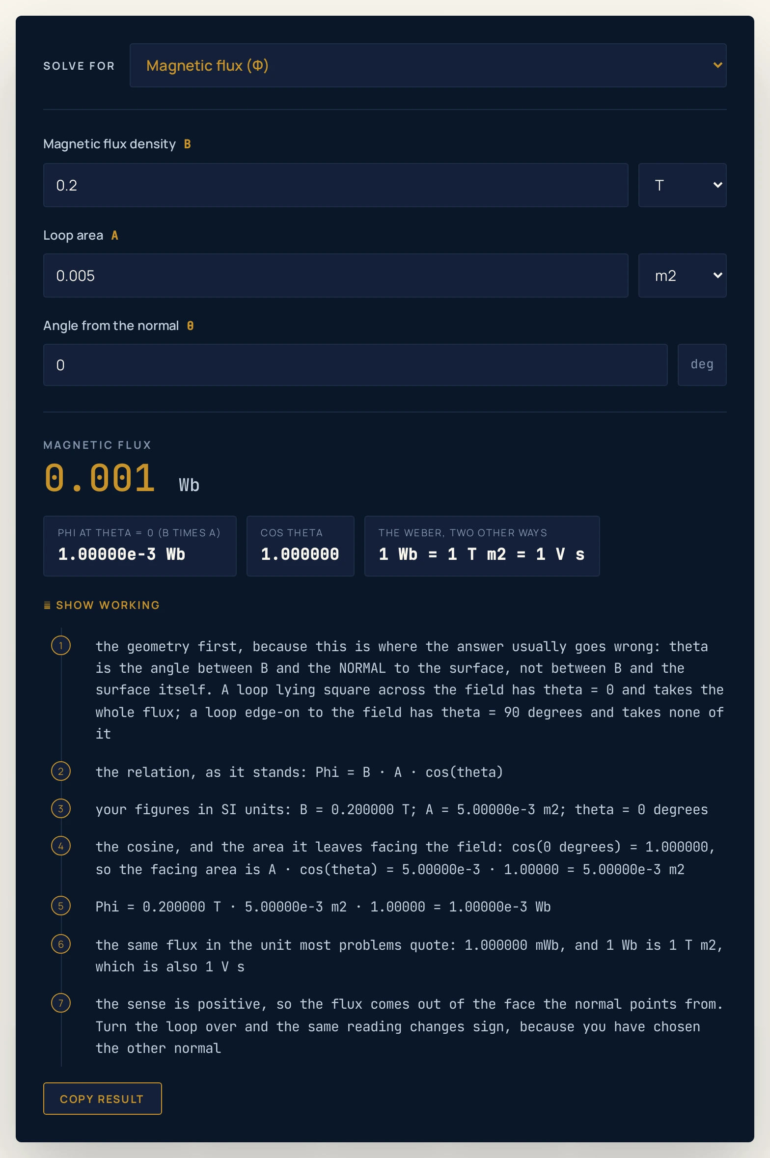
Worked example: change one thing at a time
The table starts at the defaults and moves one thing at a time: the tilt, then the field and the area together, then which quantity is the unknown, and finally two entries the calculator declines. Every Headline and chip cell was read out of the running widget rather than worked out by hand. Where a cell and the tool ever part company, believe the tool.
| Step | Solve for | What you type | Headline | Flux at zero degrees | Cosine of the angle |
|---|---|---|---|---|---|
| The page as it opens: the loop square to the field | the flux | B = 0.2 T, A = 0.005 m2, θ = 0 deg | 0.001 Wb | 1.00000e-3 Wb | 1.000000 |
| Only the tilt changed: 60 degrees from the normal | the flux | B = 0.2 T, A = 0.005 m2, θ = 60 deg | 0.0005 Wb | 1.00000e-3 Wb | 0.500000 |
| Tilted all the way to edge-on | the flux | B = 0.2 T, A = 0.005 m2, θ = 90 deg | 0 Wb | 1.00000e-3 Wb | 0.000000 |
| Flipped right over | the flux | B = 0.2 T, A = 0.005 m2, θ = 180 deg | -0.001 Wb | 1.00000e-3 Wb | -1.000000 |
| A stronger field through a smaller loop | the flux | B = 0.5 T, A = 0.001 m2, θ = 0 deg | 0.0005 Wb | 5.00000e-4 Wb | 1.000000 |
| Now the field is the unknown instead | the flux density | Φ = 0.001 Wb, A = 0.005 m2, θ = 60 deg | 0.4 T | 2.00000e-3 Wb | 0.500000 |
| And now the area is | the loop area | Φ = 0.002 Wb, B = 0.25 T, θ = 0 deg | 0.008 m2 | 2.00000e-3 Wb | 1.000000 |
| Working the tilt out from a measured flux | the angle | Φ = 0.0005 Wb, B = 0.2 T, A = 0.005 m2 | 60 deg | 1.00000e-3 Wb | 0.500000 |
| The same loop fully reversed | the angle | Φ = -0.001 Wb, B = 0.2 T, A = 0.005 m2 | 180 deg | 1.00000e-3 Wb | -1.000000 |
| A flux of exactly nothing | the angle | Φ = 0 Wb, B = 0.2 T, A = 0.005 m2 | 90 deg | 1.00000e-3 Wb | 0.000000 |
| Asking for a field through an edge-on loop | the flux density | Φ = 0.001 Wb, A = 0.005 m2, θ = 90 deg | no answer | — | — |
| Asking for a tilt that would beat the maximum | the angle | Φ = 0.002 Wb, B = 0.2 T, A = 0.005 m2 | no answer | — | — |
Rows 1 to 4 are the whole geometry in four lines, with the field and the area held still. Square on the loop takes 0.001 Wb; at 60 degrees it takes exactly half that, because cos 60 = 0.5; edge-on it takes nothing; flipped right over it takes the same size again with the sign reversed. The Flux at zero degrees chip stays at 1.00000e-3 Wb throughout, because the field and the loop have not changed — only their relative orientation has.
Row 5 is the most instructive row in the table. A 0.5 T field through a 10 cm2 loop gives 0.0005 Wb, the same flux as row 2, by a completely different route: there the tilt halved it, here the loop is a fifth of the area in a field two and a half times as strong. A flux reading on its own cannot tell you which of those you are looking at, and the chips are what tell them apart.
Rows 6 and 7 turn the question round. Given a flux of 0.001 Wb through a 50 cm2 loop tilted 60 degrees, the field must be 0.4 T; given 0.002 Wb square on in a 0.25 T field, the loop must be 0.008 m2. Notice that the area the calculator returns is the loop's true area and not the area facing the field; the working prints both.
Rows 8 to 10 solve for the tilt, which is the mode worth knowing about: a flux of half the maximum needs 60 degrees, a flux of exactly minus the maximum needs 180, and a flux of exactly nothing needs 90. Those last two are the edges a carelessly written guard would refuse, so they are in the table deliberately. The answer is the size of the tilt and not its direction, because leaning 60 degrees either way gives the same flux.
Rows 11 and 12 are declined for physical reasons rather than arithmetic ones. There is no flux density that pushes a flux through an edge-on loop, and there is no angle at which a loop takes more flux than the flux density times its area — the cosine cannot exceed 1. Both refusals print a sentence, which is more use than a number would be.
The one quantity that moves smoothly between rows 1 and 4 is the cosine, and it is worth seeing the whole sweep at the default field and loop. You can reproduce any line of this by typing the angle into the widget above, or watch it move continuously in the electromagnetic induction guide, where a changing flux is the starting point rather than the answer.
| Angle from the normal | Cosine of the angle | Headline | The same flux in milliwebers |
|---|---|---|---|
| 0 deg | 1.000000 | 0.001 Wb | 1.000000 mWb |
| 30 deg | 0.866025 | 0.000866 Wb | 0.866025 mWb |
| 45 deg | 0.707107 | 0.0007071 Wb | 0.707107 mWb |
| 60 deg | 0.500000 | 0.0005 Wb | 0.500000 mWb |
| 90 deg | 0.000000 | 0 Wb | 0.000000 mWb |
| 120 deg | -0.500000 | -0.0005 Wb | -0.500000 mWb |
| 150 deg | -0.866025 | -0.000866 Wb | -0.866025 mWb |
| 180 deg | -1.000000 | -0.001 Wb | -1.000000 mWb |
Formula and symbol reference
One relation does all the work: Φ = B A cos θ. It rearranges to B = Φ / (A cos θ), to A = Φ / (B cos θ) and to θ = arccos(Φ / (B A)), which are the four modes of the Solve for menu. There is no physical constant anywhere in it, so every figure on this page is exact arithmetic on your own numbers.
The piece that carries the geometry is A cos θ, the area facing the field. Think of the shadow the loop casts on a screen placed across the field: square on, the shadow is the whole loop; tilted, it is smaller; edge-on, it is a line with no area at all. That shadow is what the flux counts, which is why the cosine and not the sine belongs in the formula.
The unit is the weber, and 1 Wb = 1 T m2. It is also 1 V s, which is a unit identity rather than a result: deriving it would mean deriving Faraday's law, and that is not this page's job.
| Symbol | Meaning | SI unit | Values used on this page |
|---|---|---|---|
| Φ | The magnetic flux: a total through the whole surface, and the quantity this page is named after | weber (Wb) | Box takes Wb, mWb or uWb. 0.001 Wb at the defaults, 0.0005 Wb once tilted to 60 degrees, -0.001 Wb flipped right over. |
| B | The magnetic flux density: the field at a point, and the thing a tesla measures | tesla (T) | Box takes T, mT or G. 0.2 T is the default, 0.5 T the stronger-field row, 0.4 T the answer in the solve-for-field row. |
| A | The area of the flat surface the flux passes through. Its true area, not the area facing the field | square metre | Box takes m2 or cm2. 0.005 m2 is the default, which is 50 cm2; 0.008 m2 is the answer in the solve-for-area row. |
| θ | The angle between B and the normal to the surface. Not the angle to the surface itself, which is its complement | degree | Always in degrees, 0 to 180. 0 is square on, 60 halves the flux, 90 is edge-on and gives none, 180 is fully reversed. |
| A cos θ | The area facing the field: the shadow the surface casts across the field, and the only part of it the flux counts | square metre | A working value printed in the steps, never an input: 0.005 m2 at 0 degrees falls to 0.0025 m2 at 60 degrees and 0 at 90. |
The physics: why only the facing area counts
A uniform magnetic field fills space with parallel lines all pointing the same way. Hold a wire loop in it and ask how many of those lines pass through the hole: that count, properly measured, is the magnetic flux. Tilt the loop and fewer get through, not because the field weakened but because the opening presents less of itself to them.
How much less is exactly the cosine. Project the loop onto a plane at right angles to the field and the projection has area A cos θ, where θ is measured from the normal; multiply that by the flux density and you have the flux. The field is unchanged throughout, and all that moved was the geometry.
That is also where the sign comes from. Choosing a normal is choosing which face of the loop you are calling the front, and past 90 degrees the field is arriving at the back instead, so the cosine and the flux both go negative. Turn the loop right over and you get the same size of reading with the opposite sign, because nothing about the field has a sign and your choice of normal does.
The distinction between a flux and a flux density is worth pinning down, because the two words are used almost interchangeably in conversation and mean different things: B in tesla is a field at a point, while Φ in webers is a total through a surface. They are tied by 1 T = 1 Wb/m2, so the same flux through a quarter of the area is four times the density. The magnetic field calculator gives you a flux density from a winding; this page turns one into a flux.
One more property has no formula on this page but is worth knowing, because it is what makes a flux a sensible quantity at all. The net flux out of any closed surface is zero, always, because magnetic field lines have no starts and no ends — whatever goes in comes out again. Put a closed box in a uniform field and the flux in through one face exactly cancels the flux out through the opposite one.
Why does any of this matter? Because a flux that changes is what drives an EMF round a circuit, and that is Faraday's law. The Faraday's law formula guide owns that relation, and you can watch a flux swing back and forth in the electromagnetic induction simulator, whose flux readout changes because a magnet is being driven in and out at a frequency you set — it has no tilt control at all, which is exactly the gap this calculator fills.
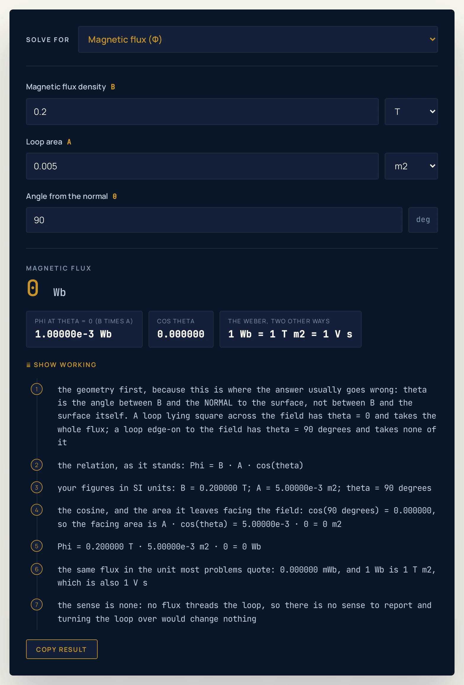
0 exactly and the facing area has fallen to 0 m2 — while the Phi at theta = 0 chip still reads 1.00000e-3 Wb, because the field and the loop have not changed.Where the magnetic flux calculator breaks down
The arithmetic here is three multiplications, so nothing fails numerically except where a division by zero is genuinely being asked for. What limits the page is the model around it: one flat surface, one uniform field, one instant in time.
- The field has to be uniform across the whole surface
- One flux density goes in, so the answer assumes the same
Beverywhere on the loop. A real magnet's field falls off with distance and curves, so a large loop near a small magnet has a different field at its edge than at its centre and this formula is only an estimate for it. Properly, the flux is an integral ofBover the surface;Φ = B A cos θis what that integral collapses to whenBis constant. Over a small enough patch, most fields are uniform enough. - The surface has to be flat
- A single angle describes a single normal, and only a flat surface has one. For a curved or folded surface the normal changes from place to place and the area has to be cut into patches, each with its own angle, and the contributions added. A cylinder's curved side in a transverse field is the standard example: no one angle describes it.
- Nothing here changes with time, so no EMF is computed anywhere on this page
- There is no time box, no rate of change and no induced voltage, in the widget or in any section above. A flux that changes drives an EMF, which is Faraday's law; that relation and its worked problems belong to the Faraday's law formula guide, and the direction the resulting current runs belongs to the Lenz's law guide. This page answers only what the flux is now.
- There is no turns box, because a flux is a property of the surface and not of the wire
- Winding the wire round twice does not change how much field passes through the hole. A coil of
Nturns multiplies this figure byNto give what the Faraday's law formula guide calls the flux linkage, which is a different quantity used for a different purpose; take the flux from here and multiply if that is what your problem wants. - A negative answer is a choice of normal, not a direction in space
- The sign tells you which way the flux threads the surface relative to the normal you picked, so it only means anything once you have said which face is the front. Flip that choice and every sign on the page flips with it. If your textbook's answer has the opposite sign to this page's, check which normal each of you chose before checking the arithmetic.
- The angle mode returns a size, not a direction of tilt
arccosgives one answer between 0 and 180 degrees, and a loop leaning 60 degrees to the left takes exactly as much flux as one leaning 60 degrees to the right. So the angle this page returns is how far from square on the surface is, with no information about which way it leans. A flux measurement alone cannot supply that, and no rearrangement of this formula can either.- A refusal means there is no answer, not that the calculator gave up
- Three combinations have no solution and are declined on purpose: a flux density or an area from an edge-on loop, where the cosine is zero and nothing divided by zero is a field or an area; and an angle for a flux larger in size than
B A, where the cosine would have to exceed 1. The cosine test is a tolerance against1e-12rather than a comparison with zero, so an angle within about6e-11degrees of 90 is refused as well: at that tolerance a flux of0.001Wb through this page's0.005m2 loop would come back as a field of2e11T, which is a division by a rounding error rather than a measurement. Every tilt further off than that,89.99degrees included, is answered normally. - The headline carries four significant figures, and the chips six
- The engine prints the answer to four significant figures, so a flux of
0.0007071Wb is a rounding of7.07107e-4Wb and the working is where to read the longer form. If you are chaining this answer into another calculation, take the figure out of the steps rather than off the headline.
Where magnetic flux is actually used
- Specifying a transformer or motor core
- Core designers work in flux per pole, in webers, and in flux density, in tesla, at the same time: the flux is what the winding has to carry and the density is what the iron can stand before it saturates and stops responding to more current. The two are the same quantity divided by an area, which is exactly the conversion this page does. Specific saturation figures depend on the alloy and the temperature — verify before use.
- Working out how much of a sensor's face is doing anything
- A flux-gate or search-coil sensor only responds to the component of field along its own axis, so mounting it a few degrees off alignment costs you the cosine of that angle. Solve for the angle here with the flux you measured and the flux you expected and you have the misalignment. At small angles the loss is small — 10 degrees costs under two per cent — which is why the cosine is a forgiving function near zero and a brutal one near 90.
- Reading a magnetic stripe or a tape head
- The head is a small loop and the signal depends on the flux through it, so the gap width, the head area and the alignment all enter through the same three symbols. The arithmetic is this page's; the device-specific numbers are not ours to quote — verify before use.
- Checking a problem's answer before checking its arithmetic
- The commonest practical use of a tool like this is auditing a figure you already have. Any flux larger in size than the flux density times the area is wrong before you look at the working, because the cosine cannot exceed 1 — that is what the Phi at theta = 0 chip is for. A flux quoted in tesla, or a flux density quoted in webers, is the other half of the same check.
- Getting from a field to a flux at all
- Most problems hand you a field, because that is what a magnet or a winding produces, and ask for something that needs a flux. Produce the field with the magnetic field calculator if it comes from a solenoid, bring it here with the area and the tilt, and you have the flux. That two-step is most of what this page gets used for.
- Seeing where the formula comes from before trusting it
- The cosine is not a fudge factor and it helps to watch it rather than take it on faith. Hold the field and the loop still, sweep the tilt and watch the flux fall to nothing at 90 degrees and come back negative beyond it — the magnetic flux guide walks through that sweep with the figures, and the angle table above is the same sweep in eight lines.
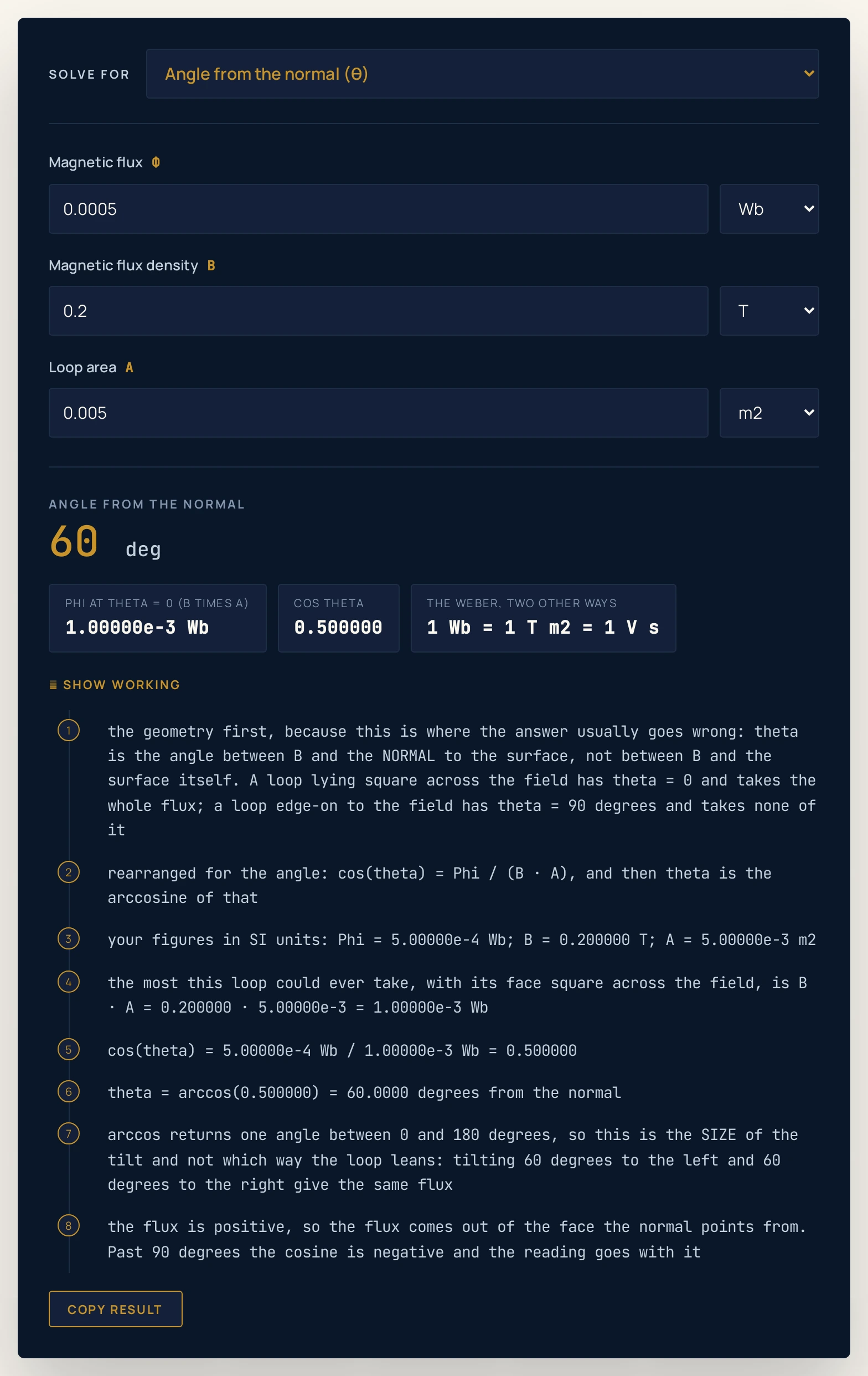
0.0005 Wb through a 50 cm2 loop in a 0.2 T field the tilt comes out at 60 degrees, and the working says plainly that this is the size of the tilt and not which way the loop leans.Where to go next
For the definition, the geometry in prose and the full set of worked problems, read the magnetic flux guide, which this tool is the arithmetic half of. The Faraday's law formula guide picks the story up where this page stops, at a flux that changes, and the electromagnetic induction guide covers the phenomenon itself. For the field that produces the flux in the first place, the magnetic field guide is the companion piece.
Four tools are worth a bookmark beside this one. The magnetic field calculator gives the flux density inside a solenoid; the magnetic force calculator gives the force on a moving charge from a speed, a field and an angle; the solenoid simulator shows the field along a real winding together with the flux through one turn; and the electromagnetic induction simulator drives a magnet in and out of a coil. The full physics lab library and the calculator index are open too.
Frequently asked questions
What does the magnetic flux calculator work out?
It works out the magnetic flux through one flat surface in a uniform field, from Phi = B times A times the cosine of theta. B is the flux density in tesla, A is the area in square metres, and theta is the angle between the field and the normal to that surface. The same relation is rearranged three more ways, so you can enter any three of the four quantities and read the fourth.
Is magnetic flux the same thing as magnetic flux density?
No, and that difference trips most people up. Flux density is the strength of the field at one point, in tesla; a flux is what gets through a whole surface, in webers, so it needs an area and a tilt before it means anything. The two meet at 1 tesla being 1 weber per square metre: one milliweber spread over the page's 50 square centimetre loop is 0.2 tesla, and over 10 square centimetres it is 1 tesla.
Why is the angle measured from the normal and not from the loop itself?
Because what matters is how much of the surface the field actually crosses, and that is the shadow the loop casts on a plane at right angles to the field. That shadow has area A times the cosine of the angle between the field and the normal. Measuring from the loop face instead gives you the complement, so the sine appears where the cosine belongs.
What happens to the flux when the loop is edge-on to the field?
It is zero: at 90 degrees from the normal the field runs along the surface instead of through it, so nothing threads the loop and the cosine is 0. The calculator returns an exact zero there rather than a tiny leftover number, because the cosine of 90 degrees really is exactly zero. The flux density is unchanged at that moment, which is the clearest demonstration that a flux and a flux density are different quantities.
What does a negative magnetic flux mean?
It means the flux threads the surface the other way relative to the normal you chose. Past 90 degrees the cosine is negative and the reading goes with it; at 180 degrees the loop has been turned right over, and the flux is the same size with the opposite sign. The sign is a bookkeeping choice about which face you called the front, not a property of the field.
What is a weber?
The weber is the SI unit of magnetic flux, and 1 weber is 1 tesla square metre. It is also 1 volt second, which is a unit identity rather than a result: this page does not derive it. School-sized loops in school-sized fields give fluxes of a few milliwebers, which is why the working prints the answer in milliwebers as well.
Can I use this for a circular loop, or only a square one?
Any flat shape at all, because the only thing the formula asks of the surface is its area. Work the area out first and type it in: a circle of radius 4.0 centimetres has an area of pi times 0.040 squared, which is 5.0265 times ten to the minus three square metres, or 50.27 square centimetres. The one restriction is that the surface must be flat and the field uniform across it.
Why does the calculator sometimes refuse to give an answer?
Because some combinations genuinely have none, and printing a number for them would be worse than saying so. No flux density and no area recover a flux through an edge-on loop, since the cosine is zero and nothing divided by zero is either of them. And no angle gives a flux larger than the flux density times the area, because the cosine can never exceed 1.
References & formula source
- Magnetic flux through a flat surface in a uniform field is computed on this page as Phi = B A cos(theta), with theta the angle between the field and the NORMAL to the surface. The weber is the SI unit of magnetic flux, and 1 Wb = 1 T m2 = 1 V s; the volt-second form is a unit identity and is not derived here.
- The cosine of an angle given in degrees is taken exactly at the multiples of 90 degrees, where the true value is exactly 1, 0 or -1. Math.cos(90 * Math.PI / 180) in double-precision arithmetic is 6.123233995736766e-17 rather than 0, which would make an edge-on loop at this page's defaults report a flux of 6.123e-20 Wb. Every other angle is handed straight to the library cosine, so 60 and 120 degrees carry their usual floating-point values; an angle entered outside 0 to 180 degrees is folded onto that range first, because the cosine is an even function.
- Every figure quoted in the prose, in the worked table and in the figure captions is a string this calculator printed for the inputs named beside it. Nothing here is a measurement made on this site, and no figure has been carried in from another page without being recomputed here first.
- This page computes a flux and nothing else. It does not compute an induced EMF, a rate of change of flux or a turns count, and it has no time input of any kind. Those belong to the Faraday law and electromagnetic induction guides, which are linked in the body.
- Halliday, Resnick and Walker, Fundamentals of Physics, chapter "Induction and Inductance", section on magnetic flux.
- Young and Freedman, University Physics with Modern Physics, chapter "Electromagnetic Induction", section on magnetic flux and the weber.
- The sign of a magnetic flux follows the choice of which way the surface normal points, and is therefore a convention rather than a property of the field. Reversing that choice reverses the sign of every flux on this page without changing any physics.
- Further reading: Magnetic flux — Wikipedia