Five sliders, one instrument and one thing measured over and over. This systematic error simulator is a free interactive lab for the part of a measurement that repeating it cannot fix: set the true value, the instrument’s zero error and gain error, how far a single reading scatters, and how many readings you average. It opens on a micrometre with a 20.000 um zero error taking nine readings of a 5.000 mm block, where the four cards answer 20.000 um, 1.333 um, 20.044 um and 1 reading.
That fourth card is the one to watch, because it prices the advice this subject is usually given. Repeat ceiling reads 1 reading on the opening state: the scatter of the mean has already fallen to the size of the bias before a second reading is taken, so the eight others change the total error by less than four tenths of a micrometre. Push Readings to its top rung and the second card falls by a factor of ten, from 4.000 um to 0.400 um, while the third moves only from 20.396 um to 20.004 um.
Systematic Error vs Random Error
One instrument, measuring one thing, over and over. Set the true value, the instrument’s zero error and gain error, how much a single reading scatters, and how many readings you take. The readings, the sample mean, the truth and the long-run mean are all drawn on one shared scale, so you can watch the mean converge — on the wrong number.
Load a real instrument
Each button presses the simulation’s own matching preset, so the five sliders are written by the lab itself and every number you then see is the lab’s. There is no mode to pick, no run button and no animation to wait for, so each press lands on a finished state almost at once.
Press the second and then the third if you only press two. They are the same instrument fault and the same scatter; the only thing that changes between them is the size of the thing being measured, and the answer changes by a factor of 1,250.
Pick one of the five instruments above, or drag the five sliders yourself.
What Is the Systematic Error Simulator?
The systematic error simulator is a free interactive physics lab that runs in your browser, with nothing to install and no sign-up. One instrument measures one thing over and over, and what comes out is drawn three times: as a cloud of readings with the truth and the long-run mean marked on the same axis, as a running mean closing onto a line, and as two bars in one error budget. The panel answers four things about the state you set and puts a sentence under each of them.
Five ladders drive it and not one of them is a free-typed number. True value steps through eight rungs from 0.0400 mm of foil to a 50.0000 mm gauge block, Zero error through eight from -20.000 um to 50.000 um, Gain error through eight from -2.00 % to 5.00 %, Scatter (1 reading) through eight from 0.500 um to 64.000 um, and Readings through eight from 1 reading to 100 readings. That is 32,768 reachable states, which is why any figure quoted about this lab can be landed on exactly rather than approached.
Both fault ladders carry an exact nought at their middle rung, and that is deliberate rather than tidy. A reader has to be able to switch one fault off and leave the other on, because the two behave completely differently: a zero error is the same amount in every reading whatever you point the instrument at, while a gain error is a percentage of the thing being measured and therefore changes size with it.
Four cards carry the answer, each with its own line underneath. Systematic error (bias) is the two faults added together and is the one term the reading count cannot touch. Random error of the mean is the scatter divided by the square root of the reading count. Total error (rms) is those two added in quadrature. Repeat ceiling is the first count at which the second has fallen to the size of the first.
The lab opens on a micrometre with a 20.000 um zero error, no gain fault and 4.000 um of scatter, taking nine readings of a 5.000 mm block, where those four read 20.000 um, 1.333 um, 20.044 um and 1 reading. A compact grid under the drawing adds eight more readings, which on that state are a truth of 5.0000 mm, a long-run mean of 5.0200 mm, a sample mean of 5.0186 mm out by 18.638 um, a bias share of 99.56 %, a relative bias of 0.40 %, 1 reading needed to see the fault at two sigma, and 4.103 um of scatter in that sample.
A one-sentence strip under the drawing is the only place the lab gives advice, and it has exactly three forms. On that opening state it reads The instrument is the limit. More readings will not help; check the zero and the gain against a standard. With both faults off it reads Your hand is the limit. More readings will help: four times as many halves this. In between it quotes the ceiling instead, as in Both terms matter here. The ceiling is 25 readings; past it, only a calibration helps. Which one you get is decided by the bias share and nothing else.
Readings is the slider the whole lab is built to argue with. Walk it from end to end on the opening instrument and the first card does not move at all: it reads 20.000 um at every one of the eight rungs. The second card falls tenfold, through 4.000 um, 2.828 um, 2.000 um, 1.333 um, 1.000 um, 0.800 um, 0.566 um and 0.400 um, and the third barely stirs, through 20.396 um, 20.199 um, 20.100 um, 20.044 um, 20.025 um, 20.016 um, 20.008 um and 20.004 um. A hundredfold increase in work bought under four tenths of a micrometre.
Two of the five preset buttons are a pair and they make the sharpest point on the panel. The same 2.00 % gain fault with the same 4.000 um of scatter is a 0.800 um bias on 0.0400 mm of foil, where the ceiling card reads 25 readings and the bias share is exactly 50.00 %; on a 50.0000 mm block it is 1.00000 mm, the ceiling is 1 reading and the share is 100.00 %. One instrument, one scatter, and a bias ratio of 1,250 decided entirely by the size of the thing measured.
A fifth preset is the twist. Give the instrument a zero error of one sign and a gain error of the other and there is exactly one length at which the two cancel: at 1.0000 mm the bias card reads 0.000 um, the long-run mean sits on the truth and the ceiling card reads no ceiling. Move the first slider alone and the same instrument is 245.000 um out at 50 mm and -4.800 um out on foil, with the sign reversing across that one honest length. A single-point calibration done there finds nothing at all.
The drawing is three labelled bands on one shared reading scale. The top band plots the readings as dots between a solid line at the truth and a dashed line at the long-run mean, with two brackets side by side beneath them through the same pixel mapping, so the length of the bias against the length of plus or minus one standard error is something you can read off by eye. Raising the reading count appends dots and never moves one already drawn, and moving a fault slides the whole cloud rigidly.
The middle band plots the running mean against the reading count on a decade-anchored logarithmic axis ticked at one, ten and a hundred only, inside an envelope of two sigma over the square root of the count. That envelope is drawn about the long-run mean and not about the truth, and the band says so in words, because watching a mean converge confidently onto the wrong number is the single most important thing this lab has to show. At a single reading there is no curve to draw and the band says so rather than standing empty.
The bottom band is the error budget, and its two bars are labelled by their sources rather than by their quantities: the instrument with its bias above your hand with the scatter over the square root of the count. Both are drawn on one shared scale in the same unit, a zero bias draws no bar at all, and a thin strip underneath marks the ceiling against the current count and says whether you are before, at or past it, or reads no ceiling when the instrument has no bias.
New sample redraws the scatter and nothing else. Press it three times on the opening state and the sample mean moves through 5.0186 mm, 5.0203 mm and 5.0230 mm while the scatter in the sample moves through 4.103 um, 3.523 um and 3.135 um — and the four primary cards print identical strings every time, because not one of them depends on which readings you happened to get. Reset restores the opening five positions and replays the settle.
What the lab does not model, stated as omissions rather than as assumptions that happen to hold: the bias is the same in every reading by construction, so a drifting fault, which both shifts the mean and inflates the apparent scatter, is not what these sliders set; the readings are independent, so every standard error printed here is the best case and a correlated run makes it optimistic with no warning in the formula; the scatter is normal, where a rounded dial makes it uniform on the resolution; and the scatter of a single reading is given here as known, where on a bench it is estimated from the sample and is itself uncertain by about a quarter of its own value at nine readings. The preset names are shorthand for the figures behind them rather than claims about any particular instrument.
| Control | Range | Step, default and what it moves |
|---|---|---|
| True value | 0.040 to 50 mm | a ladder of 8 fixed rungs - 0.040, 0.100, 0.500, 1.000, 5.000, 10.000, 25.000 and 50.000 mm - so the slider steps 1 index at a time and opens on rung 4, where the label reads "5.0000 mm". It is the size of the thing being measured, which is the one luxury a simulation has and a bench does not. It changes the bias whenever there is a gain fault and leaves it alone when there is not: at 2 per cent gain the bias runs from 0.800 um at the bottom rung to 1.00000 mm at the top |
| Zero error | -0.020 to 0.050 mm | a ladder of 8 fixed rungs - -0.020, -0.005, -0.001, 0, 0.001, 0.005, 0.020 and 0.050 mm - stepping 1 index at a time and opening on rung 6, where the label reads "20.000 um". It is added to every reading whatever the size of the thing measured, which is what an unchecked anvil or an untared balance does. The middle rung is an EXACT zero, so this fault can be switched off while the gain fault stays on |
| Gain error | -2 to 5 per cent | a ladder of 8 fixed rungs - -2, -0.5, -0.1, 0, 0.1, 0.5, 2 and 5 per cent - stepping 1 index at a time and opening on rung 3, where the label reads "0.00 %". It is a percentage of whatever is being measured, so unlike the zero error its size depends on what you point the instrument at. The middle rung is an EXACT zero. With one of these two sliders off and the other on, which fault you have is readable straight off the first slider |
| Scatter of one reading | 0.0005 to 0.064 mm | a ladder of 8 fixed rungs - 0.0005, 0.001, 0.002, 0.004, 0.008, 0.016, 0.032 and 0.064 mm - stepping 1 index at a time and opening on rung 3, where the label reads "4.000 um". The panel labels it "Scatter (1 reading)". It is the standard deviation of a single reading and the only quantity on the panel that the reading count works on, which is why it alone sets how far the dots in the top band spread |
| Readings | 1 to 100 | a ladder of 8 fixed rungs - 1, 2, 4, 9, 16, 25, 50 and 100 - stepping 1 index at a time and opening on rung 3, where the label reads "9 readings". It divides the scatter by its own square root and divides the bias by nothing at all. On the opening instrument it takes the second card from 4.000 um to 0.400 um and the third from 20.396 um to 20.004 um, and raising it appends dots in the top band rather than moving any already drawn |
| New sample and Reset | two buttons | New sample advances the seeded sample index and leaves every slider alone, so it redraws the scatter only: the sample mean, the sample error and the sample scatter move while all four primary cards print identical strings. Reset restores the opening state - 5.000 mm, a 0.020 mm zero error, no gain fault, 0.004 mm of scatter and nine readings - returns the sample index to its first pool and replays the settle, so the marker eases in rather than cutting to its place. There is no run button and no animation anywhere in this lab |
How to use the systematic error simulator
- Read the four cards before you touch anything. They are already answering for a micrometre with a
20.000 umzero error, no gain fault and4.000 umof scatter, taking nine readings of a 5.000 mm block: Systematic error (bias)20.000 um, Random error of the mean1.333 um, Total error (rms)20.044 umand Repeat ceiling1 reading. - Read the sentence strip under the drawing, because it is the only place the lab gives advice. On that state it says
The instrument is the limit. More readings will not help; check the zero and the gain against a standard.It has exactly three forms across every state, and which one you get is decided by the bias share in the grid,99.56 %here. - Compare the two brackets in the top band, not the two numbers. One runs from the solid
true 5.0000 mmline to the dashedlong-run mean 5.0200 mmline and is labelledthe bias, 20.000 um; the other is+/- SE, 1.333 umabout this sample’s mean, and it spans two standard errors because it is a plus-or-minus. Both are drawn through the same pixel mapping on purpose, so what you are reading off is a real ratio and not two pictures side by side. - Now walk Readings from end to end and watch which cards move. The first card does not move at all. The second falls from
4.000 umto0.400 um, the third from20.396 umto20.004 um, and the bias share climbs from96.15 %to99.96 %. A hundred times the readings, and the answer is still twenty micrometres out. - Put Readings on its bottom rung and look at the middle band. With one reading there is no trend to plot, so the band says
1 reading: no trend to seerather than drawing an empty frame, and the grid cell for the scatter in this sample reads a guarded0.000 umbecause one reading has no degrees of freedom to spare. - Switch the instrument off entirely: put Zero error and Gain error on their middle rungs. Both ladders carry an exact nought there, so either fault can be turned off while the other stays on. The first card goes to
0.000 um, the ceiling card tono ceiling, the verdict flips toYour hand is the limit. More readings will help: four times as many halves this.and the upper bar in the error budget stops being drawn. - With both faults off, walk Readings again. Now the total error is the standard error alone and it falls from
4.000 umto0.400 um— exactly tenfold — because there is nothing else left in the budget. This is the only condition in which the usual advice to take more readings is simply correct. - Turn the gain fault back on and move True value instead. A gain error is a percentage of what you are pointing at, so moving the first slider now moves the bias. Set
2.00 %and the bias runs from0.800 umon 40 micrometres of foil to1.00000 mmon a 50 mm block without the instrument changing at all. - Press New sample three or four times. The dots jump, this sample’s mean moves through
5.0186 mm,5.0203 mm,5.0230 mmand the scatter in this sample through4.103 um,3.523 um,3.135 um, while all four cards stay byte-identical. Nothing about the instrument depends on which readings you happened to get. - Press Reset when you have finished. It puts the five sliders back to
5.0000 mm,20.000 um,0.00 %,4.000 umand9 readings, returns the sample index to its first pool, and replays the opening settle so the marker eases in rather than cutting to its place.
Dragging is the right way to find out which readings move together and a poor way to land on a particular state, because all five controls step by whole rungs. The five preset buttons above exist for that reason, and the written systematic error guide is where the subject itself is argued from scratch, with the problems worked step by step.
One thing this panel cannot do is take a figure that is not on a rung, and it cannot run the relation backwards at all. The systematic error calculator takes typed numbers and solves in four directions, including the two questions this lab never asks: what bias a measured total error and scatter imply, and how many readings a target total error would need.
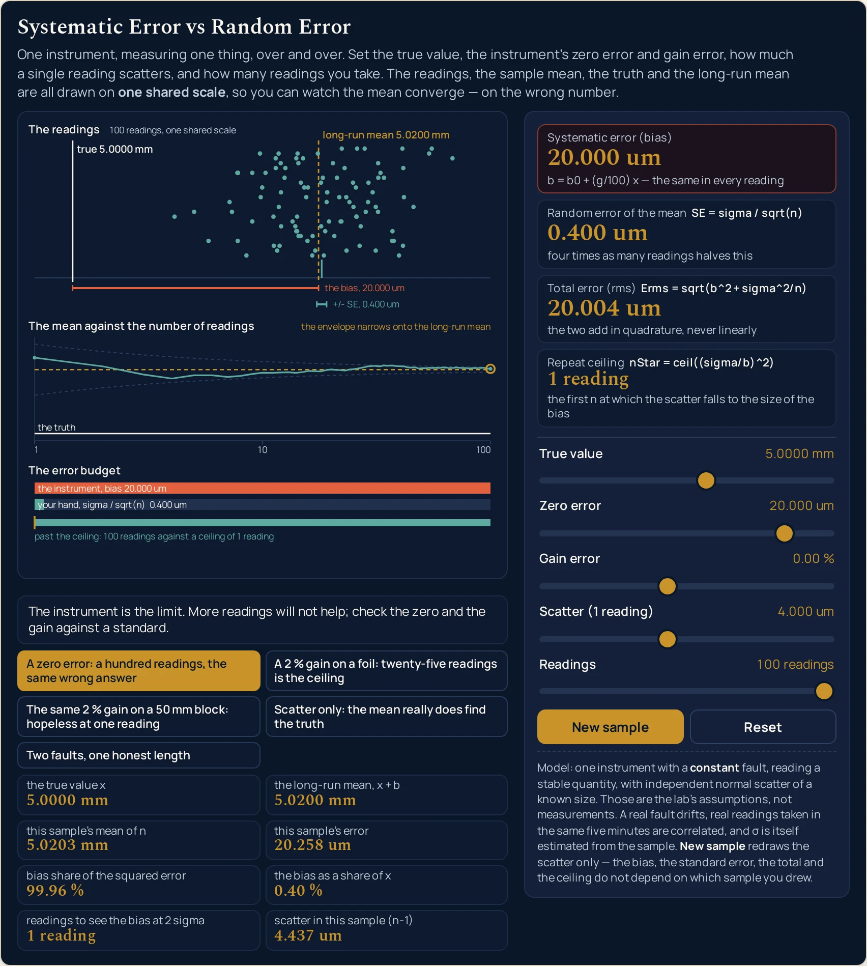
+/- SE down to 0.400 um while the bias bracket beside it is still 20.000 um long, and the total error has landed on 20.004 um. The band text here is what the drawing paints at this page’s own width; it shortens on a narrow column, band by band.Worked example: change one thing at a time
Nothing in the three tables below was worked out here. Each row is a state the lab was put into through its own controls and then read back from, cell by cell, so every string in them is the panel’s own. The first table changes exactly one slider and holds the other four still.
One: one instrument, every rung of the readings ladder
The instrument is the opening one and it never changes: a 20.000 um zero error, no gain fault, 4.000 um of scatter, measuring 5.000 mm. Only the fifth slider moves, from 1 reading to 100 readings.
| Readings | Systematic error | Random error of the mean | Total error | Bias share of the squared error | Repeat ceiling | Scatter in this sample |
|---|---|---|---|---|---|---|
| 1 reading | 20.000 um | 4.000 um | 20.396 um | 96.15 % | 1 reading | 0.000 um |
| 2 readings | 20.000 um | 2.828 um | 20.199 um | 98.04 % | 1 reading | 3.883 um |
| 4 readings | 20.000 um | 2.000 um | 20.100 um | 99.01 % | 1 reading | 4.909 um |
| 9 readings | 20.000 um | 1.333 um | 20.044 um | 99.56 % | 1 reading | 4.103 um |
| 16 readings | 20.000 um | 1.000 um | 20.025 um | 99.75 % | 1 reading | 3.649 um |
| 25 readings | 20.000 um | 0.800 um | 20.016 um | 99.84 % | 1 reading | 3.759 um |
| 50 readings | 20.000 um | 0.566 um | 20.008 um | 99.92 % | 1 reading | 4.574 um |
| 100 readings | 20.000 um | 0.400 um | 20.004 um | 99.96 % | 1 reading | 4.437 um |
The second column is the same string eight times, and that is the whole table. A hundred times the work moved the random error of the mean by a factor of ten, exactly as four times as many readings halving it requires, and moved the total error from 20.396 um to 20.004 um. The repeat ceiling said 1 reading before any of that was attempted.
The ratios behind those two numbers are asserted rather than estimated, and they are smaller than they look. Going from nine readings to a hundred — eleven times the work — removes 0.2015 per cent of the error. All hundred together, against a single reading, remove 1.9223 per cent. Under a quarter of one per cent is the honest way to say the first of those.
The last column is the one readers mistake for a fault. The scatter in this sample wobbles down the table — 3.883 um, 4.909 um, 4.103 um — because it is a sample statistic on n minus one degrees of freedom and not the setting. The setting is 4.000 um throughout. How many digits of any of these figures a written answer may keep is a separate question, and the significant figures guide is where it belongs.
Two: the five published states
These are the presets with the readings their buttons produce. Read the last two columns across: the bias share and the verdict are the two that decide whether more readings are worth taking, and they disagree completely from row to row.
| Preset | True value | Zero error | Gain error | Scatter of one reading | Readings | Systematic error | Random error of the mean | Total error | Repeat ceiling | Bias share of the squared error | What the verdict strip says |
|---|---|---|---|---|---|---|---|---|---|---|---|
| A zero error: a hundred readings, the same wrong answer | 5.0000 mm | 20.000 um | 0.00 % | 4.000 um | 100 readings | 20.000 um | 0.400 um | 20.004 um | 1 reading | 99.96 % | The instrument is the limit. More readings will not help; check the zero and the gain against a standard. |
| A 2 % gain on a foil: twenty-five readings is the ceiling | 0.0400 mm | 0.000 um | 2.00 % | 4.000 um | 25 readings | 0.800 um | 0.800 um | 1.131 um | 25 readings | 50.00 % | Both terms matter here. The ceiling is 25 readings; past it, only a calibration helps. |
| The same 2 % gain on a 50 mm block: hopeless at one reading | 50.0000 mm | 0.000 um | 2.00 % | 4.000 um | 9 readings | 1.00000 mm | 1.333 um | 1.00000 mm | 1 reading | 100.00 % | The instrument is the limit. More readings will not help; check the zero and the gain against a standard. |
| Scatter only: the mean really does find the truth | 10.0000 mm | 0.000 um | 0.00 % | 16.000 um | 100 readings | 0.000 um | 1.600 um | 1.600 um | no ceiling | 0.00 % | Your hand is the limit. More readings will help: four times as many halves this. |
| Two faults, one honest length | 1.0000 mm | -5.000 um | 0.50 % | 2.000 um | 9 readings | 0.000 um | 0.667 um | 0.667 um | no ceiling | 0.00 % | Your hand is the limit. More readings will help: four times as many halves this. |
Rows two and three are the same instrument, and they are the strongest argument on this page. Same 2.00 % gain fault, same 4.000 um scatter, and the bias goes from 0.800 um to 1.00000 mm — a factor of 1,250 — purely because the thing being measured went from 40 micrometres of foil to a 50 mm block. One of them needs 25 readings before the instrument becomes the limit; the other is beyond help at the first.
Row two is the only one of the five where the verdict strip takes its middle form. The bias is 0.800 um, the random error of the mean is 0.800 um, the share is exactly 50.00 %, and the ceiling is exactly 25 readings — so the strip under the bars reads at the ceiling rather than before or past it. It is the one state of the five where both terms genuinely matter.
Row four is the control case and row five is the twist. Row four has both faults off, so the total is the standard error alone and the ceiling card reads no ceiling. Row five has two faults that happen to cancel at the length on screen, which produces the same 0.000 um from a completely different situation — and the third table is what that one is really hiding.
Three: two faults, and the one length where they cancel
This is the fifth preset with only the first slider moved. The instrument is fixed throughout: a -5.000 um zero error, a 0.50 % gain error, 2.000 um of scatter, nine readings. Nothing about it is touched; only the size of the thing being measured changes.
| True value | Systematic error | Bias as a share of the true value | Long-run mean | Total error | Bias share of the squared error | Repeat ceiling |
|---|---|---|---|---|---|---|
| 0.0400 mm | -4.800 um | -12.00 % | 0.0352 mm | 4.846 um | 98.11 % | 1 reading |
| 0.1000 mm | -4.500 um | -4.50 % | 0.0955 mm | 4.549 um | 97.85 % | 1 reading |
| 0.5000 mm | -2.500 um | -0.50 % | 0.4975 mm | 2.587 um | 93.36 % | 1 reading |
| 1.0000 mm | 0.000 um | 0.00 % | 1.0000 mm | 0.667 um | 0.00 % | no ceiling |
| 5.0000 mm | 20.000 um | 0.40 % | 5.0200 mm | 20.011 um | 99.89 % | 1 reading |
| 10.0000 mm | 45.000 um | 0.45 % | 10.0450 mm | 45.005 um | 99.98 % | 1 reading |
| 25.0000 mm | 120.000 um | 0.48 % | 25.1200 mm | 120.002 um | 100.00 % | 1 reading |
| 50.0000 mm | 245.000 um | 0.49 % | 50.2450 mm | 245.001 um | 100.00 % | 1 reading |
Calibrate at 1.0000 mm and this instrument certifies itself as perfect. That row reads 0.000 um of bias and a long-run mean of 1.0000 mm against a truth of 1.0000 mm: the check finds nothing at all. Take the same instrument to the 25 mm standard and it reads 25.1200 mm. A one-point calibration at the wrong length is worse than no calibration, because it comes with a certificate.
The sign reverses across that length, and the two error columns disagree about where the trouble is. The absolute bias is worst at the top of the ladder, at 245.000 um; the relative bias is worst at the bottom, at -12.00 % against 0.49 %, because the fixed offset dominates where the measurement is small. The same instrument reads low on a foil and high on a block.
This is the common case rather than a curiosity. Of the 64 pairs of zero error and gain error the two middle sliders can set, 22 have a bias that changes sign somewhere across the true-value ladder, which is 34.375 per cent of them. All three of those counts come from the reference script sweeping the grid, not from a sample of it.
Formula and symbol reference
The band at the head of this page carries the total-error relation with the definition of the bias beside it, because the first on its own hides the fact that b is built from two independent faults with completely different behaviour. Every reading on the panel is one of those two expressions, a count derived from their ratio, or a share.
The symbol column below uses the panel’s own names, spelled the way the lab’s own cards spell them in plain ASCII, with sigma and sqrt written out rather than drawn. The lab switches from micrometres to millimetres at exactly one millimetre, which is why one reading can read 245.000 um and the next 1.00000 mm; the SI units guide is where those prefixes come from, and the unit conversions guide is the one to keep open if you are working in anything else.
| Symbol or readout | Meaning | SI unit | In this lab |
|---|---|---|---|
| x | The true value of the thing being measured — what a perfect instrument would read. It is a setting here rather than a reading, which is the one luxury a simulation has and a bench does not | millimetre (mm) | the first slider, a ladder of eight rungs from 40 micrometres of foil to a 50 mm gauge block, opening on 5.0000 mm. It is printed back in the grid as the true value x. Moving it changes the bias whenever there is a gain fault and leaves the bias alone when there is not, which is the cleanest way to tell the two faults apart. |
| b0 | The zero or offset error: a fixed amount added to every reading, whatever the size of the thing measured. An anvil that was never checked, or a balance never tared | millimetre (mm) | the second slider, eight rungs from -20.000 um to 50.000 um with an exact nought at the middle rung, opening on 20.000 um. With the gain slider at nought the bias card simply repeats it, which is why the opening state reads 20.000 um on both. |
| g | The gain or scale error: a percentage of whatever is being measured. A rule whose graduations are a shade too wide, or a sensor whose output is scaled slightly wrong | per cent (dimensionless) | the third slider, eight rungs from -2.00 % to 5.00 % with an exact nought at the middle rung, opening on 0.00 %. This is the fault whose size depends on what you point it at: the same 2.00 % is a 0.800 um bias on foil and 1.00000 mm on a 50 mm block. |
| b | The systematic error, which the sim calls the bias: the two faults added together, as b0 plus g over a hundred times x. It is the one term in the whole relation that does not care how many readings you take | millimetre, printed in um below 1 mm | the first card, to three decimals in micrometres below a millimetre and to five decimals in millimetres above it. 20.000 um on the opening state; 0.000 um whenever both faults are off or they exactly cancel; 2.55000 mm at the top corner of the grid. The card itself changes appearance once the bias owns at least nine tenths of the squared error. |
| sigma | The standard deviation of one reading: how far a single measurement wanders from the long-run mean. Your hand, the lighting, the anvil force, the last digit you had to judge | millimetre (mm) | the fourth slider, labelled Scatter (1 reading), eight rungs from 0.500 um to 64.000 um, opening on 4.000 um. It is the only quantity on the panel that the reading count works on, and it is also what the dots in the top band are spread by. |
| n | How many readings you take and average. The whole question this lab exists to answer is what buying more of them is worth, and the answer is almost never what the advice to repeat a measurement implies | dimensionless count | the fifth slider, eight rungs from 1 reading to 100 readings, opening on 9 readings. Raising it appends dots in the top band and never moves one already drawn, because the whole pool of standard normals is drawn once per sample and the first n of them are used. |
| sigma / sqrt(n) | The random error of the mean, usually called the standard error. It is what averaging actually buys: four times as many readings halve it, and nothing makes it fall faster than that | millimetre, printed in um below 1 mm | the second card. Down the whole reading ladder on the opening instrument it runs 4.000 um, 2.828 um, 2.000 um, 1.333 um, 1.000 um, 0.800 um, 0.566 um, 0.400 um — a fall of exactly ten over a hundredfold increase in work. At one reading its sub-line changes to say that this IS the scatter of a single reading. |
| Erms | The total error, root mean square: the bias and the standard error added in quadrature rather than head to head, because the two are independent. It is the hypotenuse of a right-angled triangle whose legs behave nothing like each other | millimetre, printed in um below 1 mm | the third card. On the same ladder it goes 20.396 um, 20.199 um, 20.100 um, 20.044 um, 20.025 um, 20.016 um, 20.008 um, 20.004 um. A hundred times the work moved the answer by less than four tenths of a micrometre, and the bracket lengths in the top band show you why before any of those numbers do. |
| nStar | The repeat ceiling: the first reading count at which the standard error has fallen to the size of the bias. Past it, the instrument is what is left and further readings are buying almost nothing | dimensionless count | the fourth card, as a phrase rather than a bare number. It reads 1 reading on the opening state, 25 readings on the foil preset, 10 readings at the low corner of the grid, and no ceiling whenever the bias is exactly nought. It never prints a figure in exponential form, by design. |
| nDet | The reading count needed to see the bias against the noise at the two-sigma level: four times the squared ratio of the scatter to the bias, rounded up. It runs about four times the repeat ceiling while the scatter is the larger of the two, so finding out that you have a fault costs roughly four times what putting up with it costs — but the two counts are rounded up separately, and both read 1 reading once the bias is at least twice the scatter | dimensionless count | the grid row labelled readings to see the bias at 2 sigma. 1 reading on the opening state, 100 readings on the foil preset where the ceiling is 25, 38 readings at the low corner, and no ceiling wherever the ceiling card says so. |
| the bias share | How much of the mean square error the instrument owns, as a percentage. It is the one number on the panel that decides whether taking more readings is worth doing at all, and the verdict strip is built from it | per cent (dimensionless) | the grid row labelled bias share of the squared error. Up the reading ladder on the opening instrument it climbs 96.15 %, 98.04 %, 99.01 %, 99.56 %, 99.75 %, 99.84 %, 99.92 %, 99.96 %. At or above 90 % the strip says the instrument is the limit; at or below 10 % it says your hand is. |
| x + b | The long-run mean: where the average of your readings is heading, which is not the truth unless the bias is nought. It is the dashed line in the top band and the centre of the envelope in the middle one | millimetre (mm) | the grid row labelled the long-run mean, x + b, and the dashed vertical line labelled long-run mean 5.0200 mm on the opening state. On the 50 mm block preset it is 51.0000 mm against a truth of 50.0000 mm, which is a whole millimetre of daylight between the two lines. |
| the correction | Subtracting the zero error and then dividing by the gain, which recovers the true value exactly in this model. It is the only thing that moves a bias at all, and there is no control for it here | not a control | not on the panel. This lab goes forwards only: you set a fault and it reports what the fault costs. Working the relation backwards — what bias a measured total error and scatter imply, or how many readings a target total error needs — is the companion calculator's job, and it has four solve modes for it. |
If you read one row twice, make it the bias share. Everything else on the panel is a quantity; that one is a decision, and the verdict strip is simply it put into words. Above about nine tenths the instrument is what is left and no reading count helps; below about a tenth your hand is, and four times as many readings really do halve what you have.
The physics: why averaging cannot touch a bias
Leave the panel on its opening state and ask what the dashed line in the top band is. It is the long-run mean, which is where the average of your readings is going: not the truth, but the truth plus the bias. The dots scatter about that dashed line and never about the solid one, and no number of dots changes which line they are scattered about.
That is the whole of it, and the middle band is the proof drawn rather than asserted. The envelope there is two sigma over the square root of the reading count, and it closes as the count rises — onto the dashed line. The running mean walks inside it, converging neatly and confidently on the wrong answer, which is why the band labels the envelope the envelope narrows onto the long-run mean instead of leaving a reader to assume otherwise.
The two terms therefore cannot be added head to head. They are independent, so they combine as the legs of a right-angled triangle, and shrinking the shorter leg barely moves the hypotenuse. That is the arithmetic behind every row of the first table: at nine readings the bias is fifteen times the standard error, and squaring both before adding is what turns a fifteen-to-one ratio into a 99.56 % share.
| Part of the drawing | What it paints | What it does not claim |
|---|---|---|
| the readings band | The top band, titled The readings. A horizontal reading axis in millimetres, a solid line at the truth labelled true 5.0000 mm, a dashed line at the long-run mean labelled long-run mean 5.0200 mm, the n readings as dots, a short tick at this sample’s mean, and two brackets drawn side by side — the bias, 20.000 um and +/- SE, 1.333 um. Beside the band title sits 9 readings, one shared scale |
it does not give the two brackets separate scales, and the whole band would be a lie if it did. They are drawn through the same pixel mapping, so their lengths may be compared by eye and that comparison is the lesson — with one thing to know before you read it, which is that the second bracket spans two standard errors because it is a plus-or-minus while the first spans the bias itself. The window is taken from the smallest and largest of the truth, the long-run mean and every reading, with a tenth of the span as margin, so it is never a fixed range: the absolute width of the band means nothing from one state to the next, and only the ratio of the two brackets does |
| the running-mean band | The middle band, titled The mean against the number of readings. The running mean of the first k readings against k, on a decade-anchored logarithmic axis ticked at 1, 10 and 100 and nothing else, inside a dashed envelope of two sigma over the square root of k. A solid line marks the truth, labelled the truth, and the envelope carries the envelope narrows onto the long-run mean |
it does not centre the envelope on the truth, and it says so in words rather than leaving you to notice. The envelope narrows onto the dashed long-run line, which is where the mean of n is really going. The band also carries no separate axis label: the only free slot on the decade row is the right-hand end where the 100 rung already sits, so the title names the axis instead. At a single reading there is no curve to draw and the band says 1 reading: no trend to see rather than standing empty |
| the error-budget band | The bottom band, titled The error budget. Two bars on one shared scale in the same unit, labelled by their sources rather than their quantities: the instrument, bias 20.000 um above your hand, sigma / sqrt(n) 1.333 um. Under them a thin strip marks the ceiling against the current count and reads, on the opening state, past the ceiling: 9 readings against a ceiling of 1 reading |
it does not claim a bar where there is no quantity. A zero bias draws nothing at all, so a zero-length bar always means exactly zero; the one-pixel floor applies only to a strictly positive value and the only distortion is sub-pixel. The strip’s wording is a claim the drawing has to honour: when it says past the ceiling the count really does exceed the ceiling, when it says at the ceiling the two are equal, and when the instrument has no bias it reads no ceiling: every reading helps instead of marking a position that does not exist |
| what the picture is for | Seeing which of the two terms you are actually fighting. A bracket beside a bracket, an envelope closing onto the wrong line, and two bars on one scale are the three arguments of this lab drawn rather than asserted, and every figure in all three is printed in the panel so the drawing can be checked instead of trusted | it is not evidence about any instrument. Every pixel is arithmetic on five slider positions and one seeded sample, so it shows the shape of a model rather than a measurement. The readings are drawn from a pinned generator and not from a bench, no reading on the page came from a real micrometre, and the lab prints its own assumptions in a fixed line under the controls rather than leaving them implied |
The repeat ceiling is an inverse square in the bias, which is the least intuitive thing on the panel. Halving the bias quadruples the count at which the scatter has fallen to meet it, so a better instrument stops rewarding repetition sooner, not later. Hold the scatter at 4.000 um and the foil preset’s 0.800 um bias gives a ceiling of 25 readings; a 1.000 um bias gives 16, doubling that to 2.000 um gives 4, and doubling again to 4.000 um gives 1.
Seeing the fault costs about four times what tolerating it costs, while the scatter is the larger of the two. The grid row for the readings needed at two sigma rounds up four times the squared ratio of the scatter to the bias; the ceiling card rounds up the same ratio squared, without the four. On the foil preset that is 100 readings against a ceiling of 25 readings — but each is rounded up on its own, so the low corner of the grid reads 38 readings against 10 readings, and the opening state reads 1 reading on both.
That asymmetry is why a bias usually goes unnoticed rather than unmeasured: the count at which it starts to dominate your answer arrives long before the count at which it becomes visible in your data. Between those two counts you are being misled by an instrument whose fault your own readings cannot yet show you.
There is exactly one escape, and it is not on this panel. A fixed offset can be divided by the number of events you measure across, which is a change of measurement design rather than of statistics: time twenty swings of a pendulum once and a stopwatch’s fixed offset is divided by twenty, where timing one swing twenty times leaves it whole. The pendulum period guide is where that case is worked, and the pendulum period calculator gives the period it is used to measure. Nothing on these five sliders can do it.
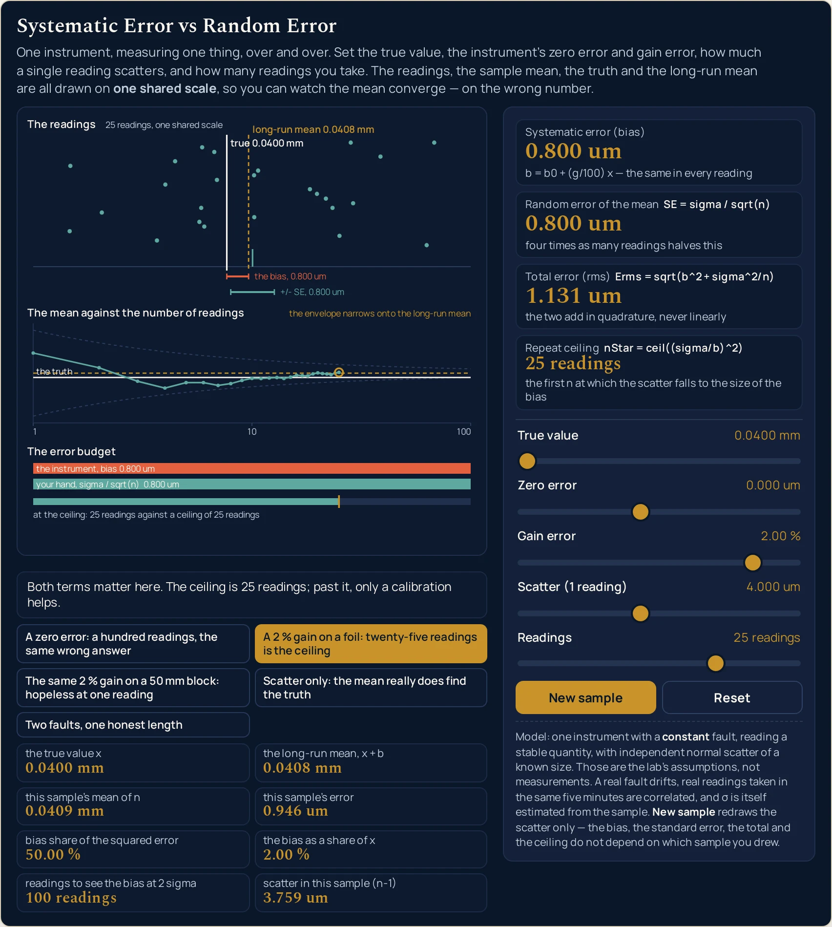
0.800 um, the share is exactly 50.00 %, and the strip underneath reads at the ceiling. Band text is as drawn at this page’s width.Where this lab breaks down
Every one of the 32,768 states the five sliders reach is answered, and the arithmetic is not where this panel can let you down. What it cannot do is model a real measurement, and what it refuses to do is treat its own idealisations as facts. The first item below matters more than the rest put together, and it is the one no competing page seems to carry.
- The random and systematic split is the right thing to learn and is not how metrology books the arithmetic
- Read this one before any of the others. The NIST summary of Technical Note 1297 classifies the components of an uncertainty by the method used to evaluate them — Type A from the statistical analysis of a series of observations, Type B by any other means — and not by whether the cause wobbles. Put the zero error on this panel into a real uncertainty budget and which category it lands in depends on how you came by the number, not on anything the instrument did. This lab draws the random and systematic picture because it is how the subject is taught and how it is understood, so do not be surprised if a calibration certificate is not written in those terms.
- Subtracting a bias does not delete it
- The same summary says a measurement equation should express a measurement process rather than simply a physical law, and that the quantities in it include the corrections. Correcting a reading therefore replaces a bias with the uncertainty of the correction, which is smaller but is not nothing. This panel takes the bias as an exact given and prints what it costs; it has no control for how well the correction itself is known, and no reading here should be read as saying a corrected measurement is exact.
- The bias here is constant, and real faults drift
- The lab’s bias is the same in every reading by construction, which is what makes it invisible to repetition. A drifting fault is not that: it both shifts the mean and inflates the apparent scatter, which is exactly why it is the easier fault to catch — the readings trend with time rather than varying randomly about a mean. A constant offset adds precisely nothing to the scatter in this sample, which is the asymmetry behind the entire subject and the reason there is no drift slider here.
- Repeats with the same instrument and the same observer cannot see the fault they share
- Nothing in the panel knows the true value except the panel. On a bench the only two routes to a fixed systematic error are measuring a quantity whose value you already know, or comparing your readings with readings made on different apparatus known to be more accurate. The first slider here is the luxury a simulation has and a bench does not, and the third table is what happens when the known quantity you chose was the one length at which your two faults cancel.
- The standard error assumes the readings are independent, and nothing warns you when they are not
- Sigma over the square root of n is a statement about independent readings. Nine measurements by the same hand in the same five minutes are correlated, and the second card is then optimistic by an amount the formula gives no hint of. There is no correlation control on this panel, so every standard error it prints is the best case. That makes the bias share printed beside it a lower bound as well, which cuts the same way: the instrument’s share of a real budget is usually larger than the figure here, not smaller.
- Sigma is set here and estimated in practice
- The fourth slider sets the scatter of a single reading as a known quantity. On a bench it is estimated from the sample itself, on n minus one degrees of freedom, and it is uncertain by roughly one over the square root of twice that — about a quarter of its own value at nine readings. The last column of the first table is that uncertainty on display: the setting is
4.000 umthroughout and the sample statistic wanders between3.649 umand4.909 umwithout the instrument changing at all. - The scatter is normal here, and a dial rounds instead
- Readings are drawn from a normal distribution. A quantised instrument does something different: rounding to the nearest step is a uniform error whose standard deviation is the step over the square root of twelve, which for a micrometre reading to a thousandth of a millimetre is about 0.2887 micrometres. That is 57.7350 per cent of the smallest scatter rung on the fourth slider and below it everywhere, so the normal model stays defensible across this panel’s whole range — but below one step of resolution a real scatter can read as exactly zero while a rounding bias is still entirely real.
- A gain error is a percentage of a quantity, and a scale has its own zero
- The third slider multiplies the true value, which is the right model for a length measured from a hard zero. It is not the right model for a reading on a scale whose zero is a convention rather than an absence of the quantity: two per cent of a temperature in degrees Celsius and two per cent of the same temperature in kelvin are different faults, and only one of them is what a sensor’s gain actually does. The absolute zero guide is where that distinction lives. Say which zero you mean before you quote a percentage.
- None of this is the limit the uncertainty principle sets
- Everything on this panel is a property of an instrument and could in principle be calibrated away. The uncertainty principle guide is about a limit nature imposes on what is simultaneously knowable, and the uncertainty principle simulator draws it in two conjugate axes. A figure count is a third thing again — a statement about how a number was written. All three limit what a measurement can tell you and no care about one of them buys anything against another.
- The sliders are ladders, and the lab runs one way only
- All five controls step by whole rungs, so the panel reaches 32,768 states and nothing between them. It also runs forwards only: you set a fault and read what it costs. There is no box to type a measured total error into and no way to ask for a bias back. Every figure on this page is arithmetic on five slider positions and one seeded sample, nothing here was measured from a real instrument, and the lab prints its own assumptions in a fixed line under the controls rather than leaving them implied.
Where the systematic error simulator is actually used
- Deciding how many readings to take before you take them
- This is the question the panel exists for, and the answer is on one card. Put your instrument’s known bias and its single-reading scatter on the second and fourth sliders and read the Repeat ceiling. At
20.000 umagainst4.000 umit is1 reading; cut the bias to a twenty-fifth and it becomes25 readings. Everything past that count is work you are doing for the look of the thing. - Working out whether a fault is even detectable with the data you have
- The grid row for the readings needed at two sigma is the one to quote when somebody asks why a known fault never showed up in their results. It is about four times the ceiling wherever the scatter is the larger of the two quantities, each count being rounded up on its own:
100 readingswhere the ceiling is25 readings, and38 readingswhere the ceiling is10 readingsat the low corner of the grid. If your run was shorter than that figure, your data was never going to see the fault, and the absence of evidence in it is not evidence of absence. - Pricing a calibration against more bench time
- Load the first preset and the trade is on screen in two cards. A hundred readings have taken the random error of the mean to
0.400 umwhile the total error sits at20.004 um, so the hundredth reading is defending four tenths of a micrometre against twenty. Checking the zero against a standard is the only thing in that picture that moves the big number, which is what the verdict strip says in words. - Catching a calibration that was done at the wrong size
- The third table is this case and it is the sharpest thing on the page. One instrument, two faults of opposite sign, and a single length at which they cancel exactly: check it there and it reads
1.0000 mmagainst a 1.0000 mm standard and passes. The same instrument is245.000 umout at 50 mm and-4.800 umout on 40 micrometres of foil. Two standards at different sizes is the cheapest defence, and 22 of the 64 fault pairs here need it. - Explaining why a careful experiment still came out wrong
- Set both faults off and the panel behaves exactly as a first course promises: the error falls tenfold from one reading to a hundred and the mean converges on the truth. Turn one fault on and it converges just as neatly on something else. The true value has to be counted in with the three fault sliders here, because a gain fault’s bias is a percentage of whatever you point it at: of the 4,096 states those four sliders reach, 152 have no bias at all, and 2,808 of the remaining 3,944 are already bias-dominated at a single reading, about seven in ten.
- Reading a quoted constant the way it was meant to be read
- Published constants come with an explicit uncertainty rather than a figure count, which is exactly the distinction this panel draws between a setting and a reading. The physics constants guide keeps the values with their uncertainties attached. Nothing on this page produces such a figure for a real instrument; it shows you what shape the budget behind one has.
- Telling an instrument problem apart from a notation problem
- If more readings do not help, the trouble is in the hardware and this panel is the picture of it. If the trouble is in how many digits a written answer is entitled to, it is a different subject with its own tools: the significant figures calculator gives the half-unit a written number claims and the significant figures simulator shows which digits of a result a figure count supports. A figure count is a coarse stand-in for precision and never the precision itself.
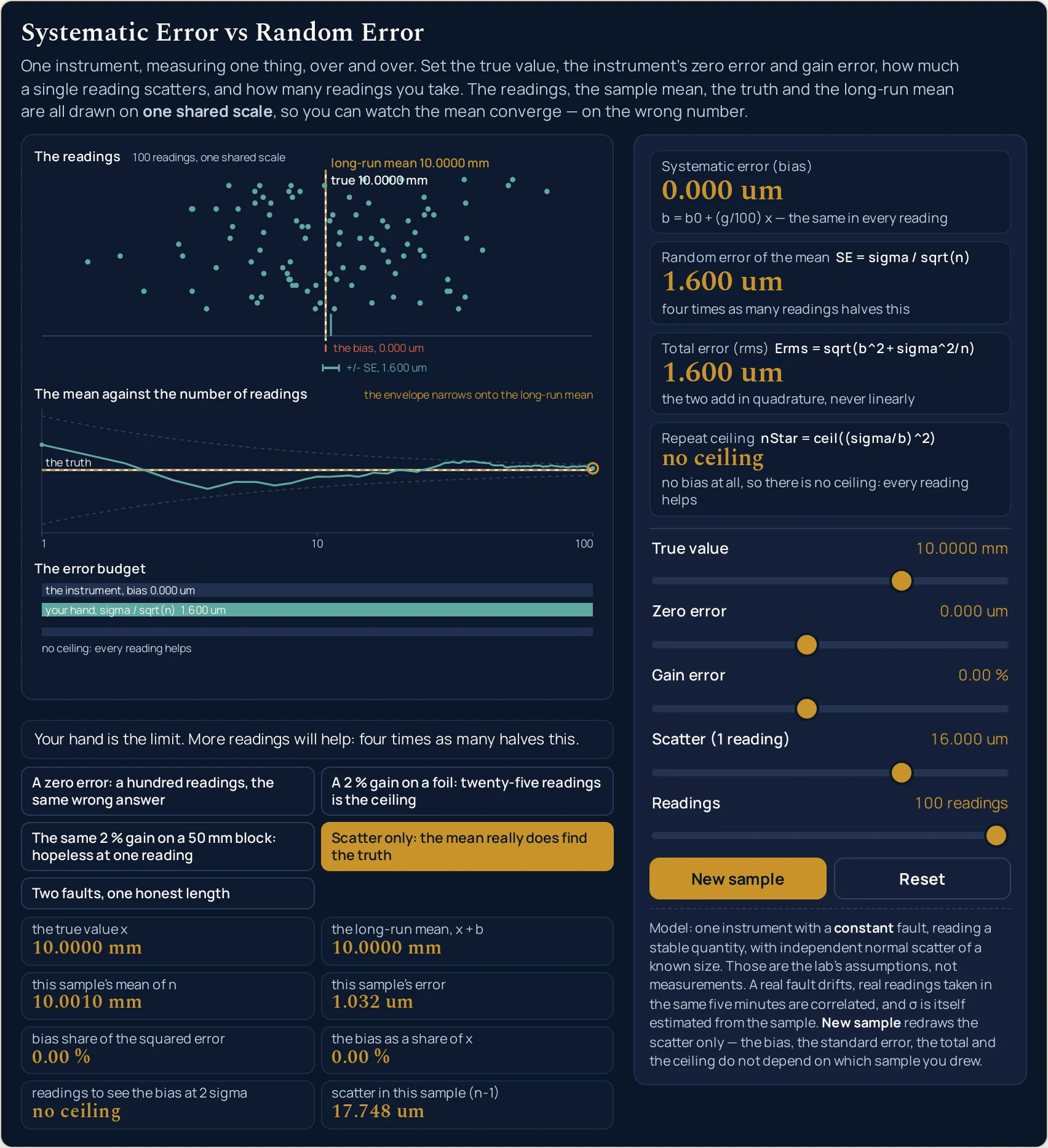
no ceiling: every reading helps, and the total error is the random error of the mean alone at 1.600 um. This is the only condition in which taking more readings is simply good advice.Where to go next
A panel can put you in a state and let you move one thing at a time, and that is the end of what a panel is for. The systematic error guide is where the subject is written out: what the two kinds of error are, why repeating a measurement cannot touch one of them, where the formal classification parts company with the teaching one, and the problems worked step by step.
Two posts own the distinctions this lab is careful not to blur. The significant figures guide is about how a number was written, and the uncertainty principle guide is about a limit nature sets rather than one an instrument does. A systematic error is a third thing again, and it is the only one of the three a calibration can do anything about.
Three more pick up what this lab uses but does not explain. The SI units guide is where the millimetre and the micrometre come from, the unit conversions guide is the one to keep open if your instrument reads in anything else, and the physics constants guide is where quoted values keep their uncertainties attached.
Two sit one step further out. The pendulum period guide carries the one classic case where a fixed offset really can be beaten, by timing twenty swings instead of averaging twenty timings, and the absolute zero guide is where the question of which zero a percentage is measured from is settled.
On the tool side, the systematic error calculator takes typed figures and solves in four directions, the significant figures calculator works on the written number, the uncertainty principle calculator gives the quantum floor, and the pendulum period calculator gives the period behind the stopwatch case.
Three neighbouring pictures sit beside this one: the significant figures simulator, the uncertainty principle simulator and the unit conversions simulator. Beyond them there is the simulation library, an index of calculators, and the blog for everything written out at length.
Frequently asked questions
Why do the four cards not move when I press New sample?
Because none of them depends on which readings you happened to get. New sample redraws the scatter only. Across sample 0, 1 and 2 at the opening state the bias, the random error of the mean, the total and the ceiling are byte-identical, while the sample mean moves through 5.0186 mm, 5.0203 mm and 5.0230 mm and the sample scatter through 4.103 um, 3.523 um and 3.135 um.
Why does the repeat ceiling read 1 reading when the page opens?
Because the bias already exceeds the scatter of a single reading, so there is nothing for a second one to improve. The opening state is a 20.000 um zero error against 4.000 um of scatter, and the ceiling is the square of the ratio of the scatter to the bias, rounded up. One reading in, the instrument is already what is left; the card beside it says so in words.
Why is the envelope in the middle band drawn about the long-run mean instead of the truth?
Because that is where the mean of n readings actually converges, and drawing it about the truth would be the central dishonesty of this subject. The envelope is two sigma over the square root of the reading count, and it narrows onto the dashed long-run line rather than onto the solid one at the true value. The band labels it in those words.
Why does the upper bar in the error budget disappear on two of the presets?
Because the bias on those two states is exactly zero, so there is no bar to draw. A zero-length bar in that band always means exactly zero: the only distortion is sub-pixel, and the one-pixel floor applies to a strictly positive quantity. Its label still prints, reading the instrument, bias 0.000 um, and the strip underneath reads no ceiling: every reading helps.
What does the thin strip under the two bars mean?
It marks the repeat ceiling against the number of readings you have set. On the opening state it reads past the ceiling: 9 readings against a ceiling of 1 reading. On the twenty-five-reading foil preset it reads at the ceiling: 25 readings against a ceiling of 25 readings. When the instrument has no bias at all it reads no ceiling: every reading helps instead.
Why do the sliders step through eight fixed rungs instead of moving smoothly?
Because a ladder makes every reading quoted about this lab reproducible rather than approximate. All five sliders are index sliders of eight rungs, which is 32,768 reachable states and nothing between them, and both the zero-error and the gain-error ladders carry an exact nought in the middle so either fault can be switched off alone. The companion calculator takes typed figures instead.
Why does the scatter in this sample read 0.000 um at one reading?
Because a sample standard deviation on one reading has no degrees of freedom, and the lab prints a guarded nought rather than a not-a-number. Set Readings to its bottom rung at the opening state and that grid cell reads 0.000 um while the random error of the mean reads 4.000 um, which is the scatter of a single reading itself. The card under it says exactly that.
Why do two presets with the same 2 % gain need such different numbers of readings?
Because a gain error is a percentage of whatever you are measuring, so the same fault is a different size on a foil and on a block. On 0.040 mm of foil the 2 % gain is a 0.800 um bias and the ceiling is 25 readings. On a 50.000 mm block it is 1.00000 mm and the ceiling is 1 reading. Same instrument, same scatter.
References & formula source
- Every figure on this page is one additive model read in different places. A single reading is the true value plus a systematic part that is the same every time plus a random part that is not; the mean of n readings therefore carries the systematic part in full and the random part reduced by the square root of n, and the two combine in quadrature because they are independent. The bias itself is a fixed offset plus a percentage of whatever is being measured. The relations are applied here rather than derived; the written guide derives them and works the problems.
- The two kinds of error and their standard treatment come from the Wikipedia article on observational error, read on 11 November 2026. Four things are quoted from it rather than paraphrased: that the model has two additive parts, a random error which may vary from observation to observation and a systematic error which always occurs with the same value when the instrument is used in the same way and in the same case; that random errors can be reduced by averaging multiple measurements while constant systematic errors cannot be removed by repeating measurements or averaging large numbers of results; that a systematic error can be either constant or related, for instance proportionally, to the actual value; and that a fixed systematic error can only be found either by measuring a known quantity or by comparing the readings with readings made using a different apparatus known to be more accurate.
- The same source states that drift is the easier fault to catch, because measurements indicate trends with time rather than varying randomly about a mean, and that random error is tied to precision while systematic error is tied to accuracy. This lab models only the constant case: its bias is the same in every reading by construction, which is exactly why no amount of repeating touches it and why a drifting fault is not what the sliders set. Nothing on this page is asserted from any source beyond that article and the one below.
- The second source is the NIST summary Essentials of expressing measurement uncertainty, read on 11 November 2026, adapted from NIST Technical Note 1297 and based on the ISO Guide to the Expression of Uncertainty in Measurement. Three things are taken from it: that components of uncertainty may be categorised according to the method used to evaluate them, Type A by the statistical analysis of a series of observations and Type B by means other than that; that every component, however evaluated, is represented by an estimated standard deviation called the standard uncertainty; and that a measurement equation should express not simply a physical law but a measurement process, and that the quantities in it include the corrections. That classification is reported as what that summary says, and it is the reason the first item of the breakdown list above exists.
- An independent reference script, written before the simulation and sharing no code with it, runs 208 checks with none failing over the whole model and prints every figure this cluster quotes. It asserts four identities across all 32,768 states the five sliders reach rather than at a point: that the bias does not depend on the number of readings; that the total error squared is exactly the bias squared plus the square of the standard error; that the repeat ceiling is the first count at which the standard error has fallen to the size of the bias; and that subtracting the zero error and then dividing by the gain recovers the true value exactly. The 0.2015 per cent and the 1.9223 per cent quoted above are two of its figures, and both were wrong in the first draft of this cluster by a factor of seven before the script was run.
- One state on the grid needs an explicit guard and it is worth knowing about. A zero error of one sign and a gain error of the other cancel exactly once as the measured value changes, and at a true value of 0.100 mm with a zero error of minus 0.005 mm and a gain error of plus 5 per cent the subtraction leaves a floating-point remainder of about 8.7 in ten thousand million million million rather than a clean nought. Dividing the scatter by that remainder and squaring gives a repeat ceiling of roughly 3.3 hundred thousand million million million million readings, which is an arithmetic artefact and not a fact about measurement, so the simulation snaps any bias below one part in a thousand million million of the largest figure in play to exactly nought and the ceiling card then reads no ceiling.
- The dots are not decoration and they are not random each time you look. A pinned generator draws one pool of a hundred standard normals per sample index, and the first n of them are used, so raising the reading count appends dots without moving one already on screen, and moving any of the three instrument sliders slides the whole cloud rigidly rather than reshuffling it. The pool is fixed byte for byte in the cluster specification precisely so that no other generator could pass the tests, and the first five draws of sample zero are asserted as exact strings. New sample advances the sample index; it changes this sample mean, this sample error and this sample scatter, and it changes none of the four primary cards.
- The simulation was gated before this page was written: a reference oracle at 208 checks with none failing, a Node tier at 250 checks with none failing, a headless Chrome tier at 191 checks with none failing, a mutation pass that killed 99 of 105 planted faults with none of the six survivors unexplained, a height pass at a measured maximum of 947 pixels against a 1000 pixel ceiling, and a cross-browser pass comparing 199 readout values in Chrome and Firefox at four widths with every one identical. The cluster simulation report records every one of those, and the three screenshots and every table cell on this page were read back out of the running simulation rather than computed here.
- What was not verified, stated as a gap rather than left to be assumed. Safari and WebKit: the build on the machine this was tested on will not start, so Safari was never exercised and nothing on this page is evidence about it. Assistive technology: every slider carries a label and a live value text and the drawing carries a full description of all three bands, but no screen reader was driven and no real touch target was pressed. Sample indices beyond the third: the generator is pinned for the first two and three were harvested, so higher ones were exercised only through their own clamp. And the webfonts as a reader gets them, since there are no system faces on the test machine and the exact pixel widths a reader sees were not measured.
- Nothing on this page is a measurement of any real instrument, and the preset names are shorthand for the figures behind them rather than claims about any particular micrometre, foil or gauge block. The model is one instrument with a constant fault, reading a stable quantity, with independent normal scatter of a known size; a real fault drifts, real readings taken in the same five minutes are correlated, the scatter is itself estimated from the sample, and a gauge block has a temperature coefficient. Verify any figure against your own instrument and your own standard before you use it for anything that matters.
- Further reading: Observational error — Wikipedia