The resonance simulator is a free interactive lab in which a fixed 2.00 N push is the one thing you cannot change. Four sliders set the mass, the spring, the damping and the frequency you push at; eight readings answer, and the first of them will not move however far you drag the damping slider. What the damping does move is the size of the response — by a factor of 100 across that slider alone — which is the half of resonance that decides whether a real machine survives it.
Resonance: One Oscillator, One Drive, One Response Curve
A block on a spring against a wall, pushed back and forth by a shaker at a frequency you choose. Set the mass, the spring, the damping and the drive, and watch two things. The spring and the mass alone fix the oscillator's own frequency, f0 = (1/2pi) sqrt(k/m). The damping alone fixes how big the response gets at that frequency — drive it at f0 and the swing is exactly Q times what the same steady push would give. The drive force is a fixed 2.00 N and is not a control, because the lesson is that a small force can produce a large response. Everything printed is the steady state, to four significant figures; nothing here is a claim about how long the build-up takes, and the drawn cycle takes the same two seconds whatever the drive frequency, so the strip shows the size and the timing within a cycle of the response, never its rate.
Load a real oscillator
Each button writes the four sliders and touches nothing else, which is exactly what your own hand would do. The first five hold the spring, the mass and the drive fixed and walk the damping from light to past the threshold; the last two move the drive and the spring instead.
Press the first five in order and watch two columns of the panel at once. Natural frequency f0 stays on 1.592 Hz through every one of them, while Amplitude A falls 500.0, 100.0, 10.00, 7.143, 7.042 mm. The fourth and fifth sit side by side as buttons but 0.4 N s/m apart on the damping slider, which is two of its steps, and somewhere in that gap Peak at stops being a frequency.
Pick one of the seven oscillators above, or drag the four sliders yourself.
What Is the Resonance Simulator?
The resonance simulator is a free interactive physics lab that runs in your browser, with nothing to install and no sign-up. A block sits on a spring against a hatched wall, and a shaker pushes it back and forth at a frequency you choose. Four sliders set the mass, the spring constant, the damping and the drive frequency; four cards answer with the natural frequency, the drive frequency, the amplitude and the quality factor.
The push itself is not a control. A fixed 2.00 N drives the block at every setting, which is the one restriction that makes the lab worth opening: a force slider would let anyone reach a large swing the uninteresting way. What the panel is for is the multiplier between that 2.00 N and the swing it produces, and the multiplier is where the physics lives.
One card refuses to move, and it is the first one. Hold the mass and the spring still and drag Damping (N s/m) from 0.4 N s/m to 40.0 N s/m, the full width of the slider: Natural frequency f0 reads 1.592 Hz at every step, and its sub-line stays byte-identical at f0 = (1/2pi) sqrt(k/m) — set by the spring and the mass only. Only the spring and the mass can move it, and the slider that looks most like it should cannot.
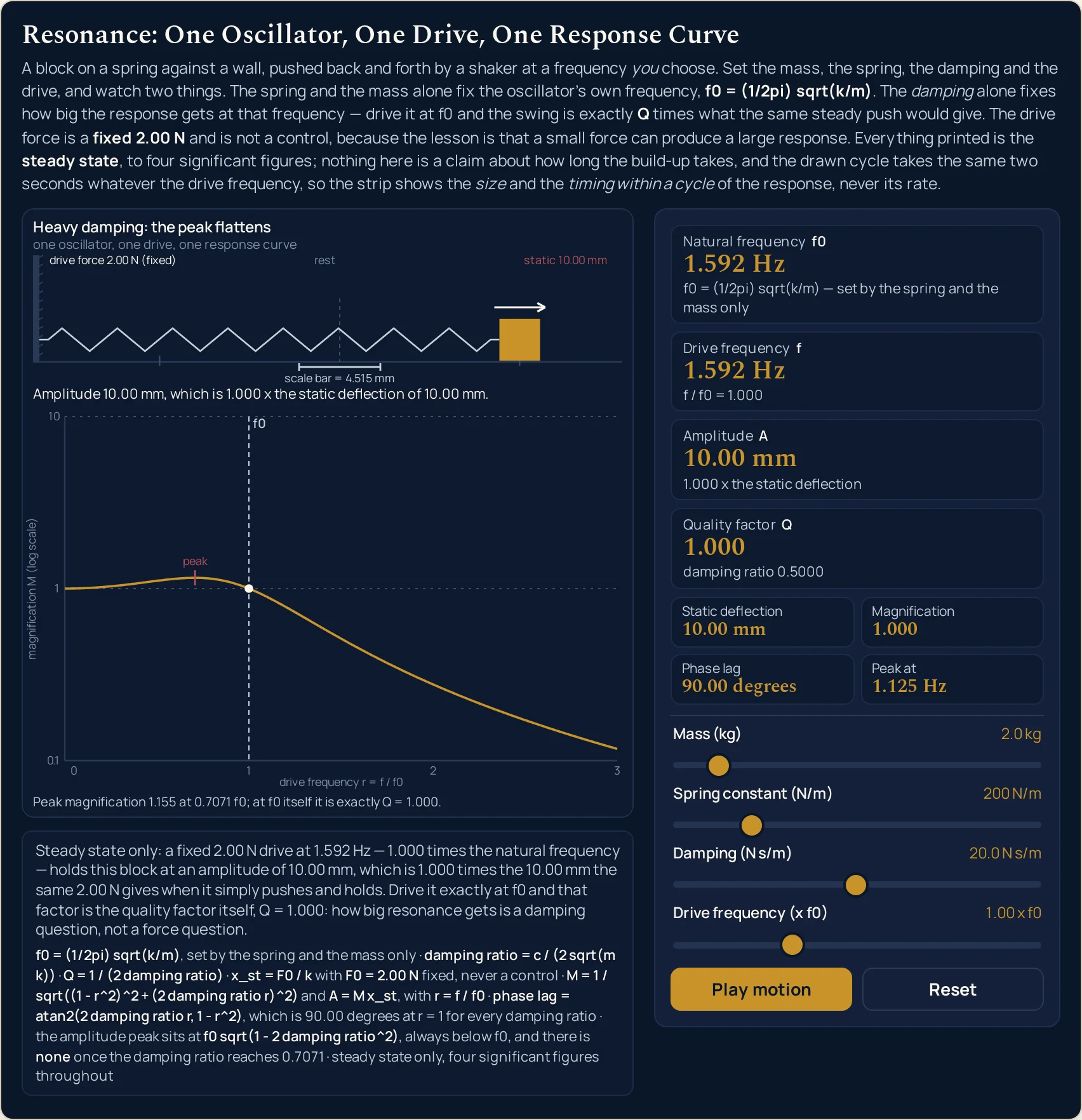
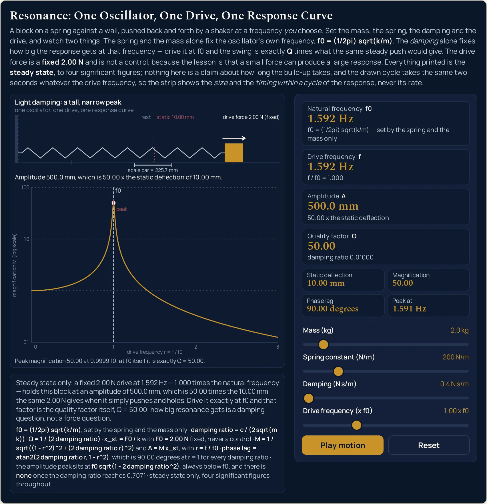
What the damping does move is the size of everything else. At 0.4 N s/m the Amplitude A card reads 500.0 mm with Quality factor Q at 50.00; at 20.0 N s/m, from the same spring, the same mass and the same drive, it reads 10.00 mm with Q at 1.000. That is a factor of 50 in the swing with nothing touched but the damper, and it is the sentence the whole lab exists to make checkable.
A compact row of four more readings sits under the cards. Static deflection is how far the same 2.00 N bends the spring when it simply pushes and holds, 10.00 mm at the opening setting; Magnification is the amplitude divided by it; Phase lag is how far the block runs behind the push; and Peak at is the frequency at which the response is actually largest. The amplitude card is simply the static deflection multiplied by the magnification, which is why there is no force box anywhere on the panel.
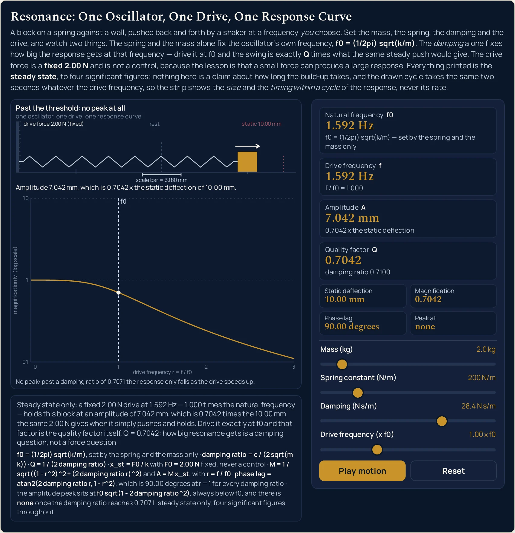
Two of those four are the awkward truths. Phase lag reads 90.00 degrees whenever the drive sits exactly on the natural frequency, for every damping value the slider reaches, with no approximation in it. Peak at reads a frequency a little below the natural one — 1.588 Hz against 1.592 Hz at the opening setting — and once the damping ratio reaches 0.7071 it prints the word none instead of a number, because there is then no peak anywhere to report.
Seven preset cases on the landing page write the four sliders for you, and two of them are deliberately 0.4 N s/m apart in the damping, which is two steps of that slider. Just inside the threshold sets 28.0 N s/m and Past the threshold: no peak at all sets 28.4 N s/m: they sit next to each other as buttons, and pressing one after the other is the only way to watch the Peak at reading stop being a frequency. The pair Light damping and Heavy damping hold the spring, the mass and the drive fixed and change only the damper.
Two sentences under the drawing do the work a card cannot. The first rewrites itself at every setting and reads the whole state back as prose, naming the fixed 2.00 N, the drive in hertz and as a ratio, the amplitude, the static deflection and the quality factor in one breath. Below it a fixed line gives the seven relations the lab uses, written in plain ASCII so that no radical and no subscript glyph is ever needed.
The drawing is a side view in two stacked panels rather than a plot against time. The upper one is the oscillator itself, drawn at its steady-state displacement with the drive arrow above it; because the reachable amplitude spans four decades the strip auto-fits, and a short scale bar states its own value in millimetres, which is what makes that auto-fitting honest. The lower panel is the response curve: the magnification against the drive frequency, with the magnification axis logarithmic and anchored on the powers of ten.
The motion runs from the moment the lab loads and the Motion button pauses it, so the button reads Pause motion on arrival rather than asking to be started. Nothing the animation touches reaches any readout: all eight readings are worked out from the four slider values alone. Every computed figure is given to four significant figures with the trailing zeros kept, and every one of them is the steady state — the lab says nothing about how long the build-up takes.
| Control | Range | Step, default and what it moves |
|---|---|---|
| Mass | 0.1 to 20.0 kg | step 0.1 kg; opens at 2.0 kg. The part that actually moves. Raising it lowers the natural frequency and raises the quality factor at the same time, because both the frequency and the damping ratio are worked out from the mass and the spring together |
| Spring constant | 10 to 1000 N/m | step 10 N/m; opens at 200 N/m. The stiffness. Four times the stiffness doubles the natural frequency, from 1.592 Hz to 3.183 Hz, and quarters the static deflection, from 10.00 mm to 2.500 mm |
| Damping | 0.4 to 40.0 N s/m | step 0.2 N s/m; opens at 2.0 N s/m. The slider that cannot touch the natural frequency and decides everything else. On the opening spring and mass its full width takes the magnification at resonance from 50.00 down to 0.5000, and from 28.4 N s/m upwards the peak reading becomes the word none |
| Drive frequency | 0.10 to 3.00 x f0 | step 0.01; opens at 1.00. A MULTIPLE of the natural frequency rather than a frequency in hertz, so that 1.00 is an exact grid point for every mass and spring. Card 2 prints the hertz it works out to, 1.592 Hz at the opening setting |
| Motion | runs from load; pauses | one button, and the motion is already running when the lab loads, so the button starts out reading Pause motion. Pressing it freezes the frame. Nothing the motion touches reaches any readout, so pausing changes no reading at all |
| Reset | back to the opening setting | one button; it restores all four sliders to 2.0 kg, 200 N/m, 2.0 N s/m and 1.00 x f0, and leaves the motion running |
How to use the resonance physics simulator
- Read the eight readings before you touch anything. The four cards are already answering for a 2.0 kg block on a 200 N/m spring pushed at its own frequency: Natural frequency f0 1.592 Hz, Drive frequency f 1.592 Hz, Amplitude A 100.0 mm and Quality factor Q 10.00. The compact row under them reads 10.00 mm, 10.00, 90.00 degrees and 1.588 Hz.
- Notice what is missing from the panel: there is no force control. The push is a fixed
2.00 Nat every setting, and the sentence strip under the drawing says so outright. That single restriction is what makes the Amplitude card worth reading: 100.0 mm of swing from a push that bends this spring 10.00 mm when it just leans on it. The resonance in physics guide is where that mechanism is argued out cycle by cycle; this panel only ever shows you the result. - Now drag Damping (N s/m) and nothing else, and keep your eye on the first card. Take it to
0.4 N s/mand the Amplitude card reads 500.0 mm; take it to20.0 N s/mand it reads 10.00 mm. Through both of those the Natural frequency card has not moved off 1.592 Hz, and neither has its sub-line. - Then move Drive frequency (x f0) instead, and watch the opposite happen. This slider is a multiple of the natural frequency rather than a frequency in hertz, so
1.00is exactly on resonance whatever the first two sliders say. Push it to2.00and the amplitude collapses from 100.0 to 3.326 mm — while Quality factor sits there reading 10.00 in both states. - Read the Phase lag cell while you do it. It is the one reading that marks the natural frequency exactly, and it is savage about it: 78.63 degrees at
0.99 x f0, 90.00 degrees at1.00, 101.3 degrees at1.01. One step of the slider either side, and the quarter-cycle lag is gone. - Move Mass (kg) and Spring constant (N/m) to see the first card finally respond. Four times the stiffness takes it from 1.592 to 3.183 Hz; four times the mass takes it the other way to 0.7958 Hz. These are the only two controls it answers to. The spring constant calculator is where the stiffness you type in here is measured from a load and an extension.
- Read the drawing in two halves, and read the scale bar first. The upper strip is the block at its steady swing; the lower panel is the whole response curve with your drive marked on it by a filled dot. The strip auto-fits, so the block never looks much bigger or smaller than it did — the short bar underneath it prints the millimetres that make the picture honest.
- Press Pause motion when you would rather read than watch. The motion is already running when the page loads, so the button reads Pause motion rather than asking to be started, and pressing it changes no reading at all. Reset puts all four sliders back to
2.0 kg,200 N/m,2.0 N s/mand1.00 x f0and leaves the motion running.
Dragging is the right way to find out which readings a control is allowed to move, and a poor way to hit an exact figure — the mass slider steps in tenths of a kilogram, the spring in tens of newtons per metre and the damping in fifths. When you already know the stiffness and the mass and want the frequency typed out to four figures, the resonance frequency calculator does that step, and solves it backwards for the mass or the spring as well. It has no drawing and no millimetres; this panel has no unit menus.
Worked example: change one thing at a time
Nothing in the three tables below was worked out here. Each row is a setting the lab was put into and then read back from, cell by cell, so every string in them is the panel’s own. Each table moves exactly one slider down its column and pins the other three, which is what makes the column that changes diagnostic.
One: the damping slider, with everything else pinned
The mass stays at 2.0 kg, the spring at 200 N/m and the drive at 1.00 x f0 in all seven rows. Only the damper changes, from the floor of its slider to its ceiling.
| Damping slider | Natural frequency | Quality factor | What the sub-line says | Amplitude | Magnification | Phase lag | Peak at |
|---|---|---|---|---|---|---|---|
| 0.4 N s/m | 1.592 Hz | 50.00 | damping ratio 0.01000 | 500.0 mm | 50.00 | 90.00 degrees | 1.591 Hz |
| 2.0 N s/m | 1.592 Hz | 10.00 | damping ratio 0.05000 | 100.0 mm | 10.00 | 90.00 degrees | 1.588 Hz |
| 6.0 N s/m | 1.592 Hz | 3.333 | damping ratio 0.1500 | 33.33 mm | 3.333 | 90.00 degrees | 1.555 Hz |
| 20.0 N s/m | 1.592 Hz | 1.000 | damping ratio 0.5000 | 10.00 mm | 1.000 | 90.00 degrees | 1.125 Hz |
| 28.0 N s/m | 1.592 Hz | 0.7143 | damping ratio 0.7000 | 7.143 mm | 0.7143 | 90.00 degrees | 0.2251 Hz |
| 28.4 N s/m | 1.592 Hz | 0.7042 | damping ratio 0.7100 | 7.042 mm | 0.7042 | 90.00 degrees | none |
| 40.0 N s/m | 1.592 Hz | 0.5000 | damping ratio 1.000 | 5.000 mm | 0.5000 | 90.00 degrees | none |
Read the second column down the page first. 1.592 Hz in all seven rows, from the lightest damping the slider offers to a hundredfold more of it. The damper is the control that looks most like it ought to change the frequency, and it is the one control that cannot.
Now read the amplitude column beside it. 500.0, 100.0, 33.33, 10.00, 7.143, 7.042, 5.000 mm — a factor of 100 from the same spring, the same mass and the same 2.00 N. Rows one and four are the pair worth pressing one after the other: Light damping and Heavy damping differ in nothing but the damper, and the swing between them differs by 50.
The last three rows are where the panel stops reporting a peak. At 28.0 N s/m Peak at still prints 0.2251 Hz, which looks like an answer; its magnification is 1.000, the same as a drive of nothing at all, so there is nothing there to find. The slider stop between that row and the next, 28.2 N s/m, is still inside the threshold at a damping ratio of 0.7050 and still prints a frequency, 0.1228 Hz. Only at 28.4 N s/m — two steps from 28.0, 0.4 N s/m more damping — does the reading become the word none, and it stays that word to the end of the slider.
Two: the spring and the mass, which are the only controls the first card answers to
The damper stays at 2.0 N s/m and the drive at 1.00 x f0. Rows one to three move the spring alone; rows four and five move the mass alone, around the same middle row.
| Mass slider | Spring slider | Natural frequency | Static deflection | Quality factor | Amplitude | Peak at |
|---|---|---|---|---|---|---|
| 2.0 kg | 50 N/m | 0.7958 Hz | 40.00 mm | 5.000 | 200.0 mm | 0.7878 Hz |
| 2.0 kg | 200 N/m | 1.592 Hz | 10.00 mm | 10.00 | 100.0 mm | 1.588 Hz |
| 2.0 kg | 800 N/m | 3.183 Hz | 2.500 mm | 20.00 | 50.00 mm | 3.181 Hz |
| 0.5 kg | 200 N/m | 3.183 Hz | 10.00 mm | 5.000 | 50.00 mm | 3.151 Hz |
| 8.0 kg | 200 N/m | 0.7958 Hz | 10.00 mm | 20.00 | 200.0 mm | 0.7953 Hz |
Rows one to three are a factor of sixteen in stiffness and a factor of four in frequency. 50, 200, 800 N/m give 0.7958, 1.592, 3.183 Hz. The static deflection goes the other way and faster — 40.00, 10.00, 2.500 mm — because a stiffer spring bends less under the same fixed push.
Rows four and five do it with the mass and reach the same two frequencies. 0.5 kg gives 3.183 Hz and 8.0 kg gives 0.7958 Hz, matching rows three and one exactly — and the static deflection stays at 10.00 mm in both, because the spring has not been touched. Two different controls, the same frequency, a different panel underneath it. The free, undriven version of this oscillator is next door at the simple harmonic motion simulator, and the motion itself is simple harmonic motion.
Watch the quality factor column while you do it, because it moves for a reason that is easy to miss. Nothing changed the damper, yet Q goes 5.000, 10.00, 20.00 down the spring rows and 5.000, 20.00 on the mass rows. The damping ratio is the coefficient divided by twice the square root of the mass times the spring, so raising either of those raises that root and lowers the ratio — and Q is one over twice the ratio, which is why it climbs as the ratio falls.
Three: the drive slider, with the oscillator left alone
Now the mass, the spring and the damper are all pinned at 2.0 kg, 200 N/m and 2.0 N s/m, and only the drive moves, from the bottom of its slider to the top.
| Drive slider | Drive frequency | Amplitude | Magnification | Phase lag | Natural frequency |
|---|---|---|---|---|---|
| 0.10 x f0 | 0.1592 Hz | 10.10 mm | 1.010 | 0.5787 degrees | 1.592 Hz |
| 0.50 x f0 | 0.7958 Hz | 13.30 mm | 1.330 | 3.814 degrees | 1.592 Hz |
| 0.90 x f0 | 1.432 Hz | 47.57 mm | 4.757 | 25.35 degrees | 1.592 Hz |
| 0.99 x f0 | 1.576 Hz | 99.03 mm | 9.903 | 78.63 degrees | 1.592 Hz |
| 1.00 x f0 | 1.592 Hz | 100.0 mm | 10.00 | 90.00 degrees | 1.592 Hz |
| 1.01 x f0 | 1.607 Hz | 97.11 mm | 9.711 | 101.3 degrees | 1.592 Hz |
| 1.10 x f0 | 1.751 Hz | 42.18 mm | 4.218 | 152.4 degrees | 1.592 Hz |
| 2.00 x f0 | 3.183 Hz | 3.326 mm | 0.3326 | 176.2 degrees | 1.592 Hz |
| 3.00 x f0 | 4.775 Hz | 1.249 mm | 0.1249 | 177.9 degrees | 1.592 Hz |
The phase column is the one to read, and it is the reason this table exists. It climbs from 0.5787 to 177.9 degrees across the slider and passes through 90.00 degrees at exactly one place, 1.00 x f0. Unlike the peak, that crossing does not move when you change the damper, which is why it is the honest signature of the natural frequency.
The amplitude column tells the other half of the story. Below resonance the block barely amplifies anything — 10.10 mm at 0.10 x f0, against a static deflection of 10.00 mm. Above it the response dies off faster than it grew: 3.326 mm at twice the natural frequency and 1.249 mm at three times it, both less than simply pushing and holding.
Rows four to six are one step of the slider either side of resonance. 0.99, 1.00, 1.01 give 9.903, 10.00, 9.711 for the magnification — barely a change. Now press Light damping and repeat it: the same three positions give 35.62, 50.00, 35.09. A tall peak is a narrow one, and one hundredth of the natural frequency is enough to fall off it.
Formula and symbol reference
The lab prints its own relations under the drawing, in the fixed definition line, in plain ASCII so that no radical sign and no subscript glyph is ever needed. Written out the same way, with sqrt spelled and every subscript an underscore:
f0 = (1/2pi) sqrt(k/m) is the natural frequency; damping ratio = c / (2 sqrt(m k)) and Q = 1 / (2 damping ratio) are the two dimensionless numbers; x_st = F0 / k is the static deflection with F0 = 2.00 N fixed; and with r = f / f0 the response is M = 1 / sqrt((1 - r^2)^2 + (2 damping ratio r)^2) with A = M x_st. Put r = 1 into that and everything but the damping term disappears, which is where M = Q comes from.
The spring constant is an input here and this panel never measures it. If you do not have a figure for the spring in front of you, the spring constant lab is where a load and an extension become a stiffness, and the Hooke’s law calculator is the force-extension relation it rests on. The amplitude this panel reports is an output and only an output; the amplitude guide is where the height of a vibration is a subject in its own right.
Fourteen rows follow and only four of them are something you drag. The rest are cards, cells of the compact row, or quantities the panel names without giving you a control for. For the sliders the right-hand column gives the end stops and the step; for everything else it gives the strings the lab prints and the span it prints them over.
| Symbol or reading | Meaning | SI unit | In this lab |
|---|---|---|---|
| f0 | The oscillator’s own frequency — the first card, labelled Natural frequency f0. A pure function of the spring and the mass, and of nothing else on the panel |
hertz | from 0.1125 Hz at 20.0 kg on 10 N/m to 15.92 Hz at 0.1 kg on 1000 N/m, the two opposite corners of the first two sliders. The sub-line under it reads f0 = (1/2pi) sqrt(k/m) — set by the spring and the mass only at every setting either of the other two sliders can reach. |
| f | The frequency the shaker is actually pushing at — the second card, Drive frequency f. You set it as a ratio; this card is where it becomes hertz |
hertz | from 0.01125 Hz to 47.75 Hz across the grid, which is more than three and a half decades. Its sub-line repeats the ratio you chose, f / f0 = 1.000 at the opening setting and f / f0 = 3.000 at the top of the drive slider. |
| r | The drive frequency as a multiple of the natural one — the fourth slider, and the only control that is a pure number | a ratio, so no unit | 0.10 to 3.00 in steps of 0.01, opening at 1.00. The chip above it prints 0.10 x f0 and 3.00 x f0 at the ends. It is a ratio rather than a frequency so that 1.00 is an exact grid point whatever the mass and the spring are set to. |
| m | The mass that moves — the first slider. Raising it lowers the natural frequency and raises the quality factor at the same time | kilogram | 0.1 to 20.0 kg in steps of 0.1, opening at 2.0 kg. Taking it from 2.0 kg to 8.0 kg alone halves the first card from 1.592 Hz to 0.7958 Hz and doubles the fourth from 10.00 to 20.00. |
| k | The spring constant — the second slider, and the one the static deflection depends on by itself | newton per metre | 10 to 1000 N/m in steps of 10, opening at 200 N/m. Four times the stiffness doubles the first card to 3.183 Hz and quarters the static deflection to 2.500 mm, because one goes as the square root of the stiffness and the other as one over it. |
| c | The damping coefficient — the third slider. The resisting force per unit of speed, and the only control the first card ignores | newton second per metre | 0.4 to 40.0 N s/m in steps of 0.2, opening at 2.0 N s/m. The floor is deliberately above zero: a zero damping would make the quality factor and the response at the natural frequency genuinely infinite, which nothing real is. |
| F0 | The peak size of the driving push. Fixed at 2.00 N and not a control at all — the lab states that in the sentence strip and the definition line under the drawing | newton | the same 2.00 N at every one of the settings on this page. A force slider would let a reader reach a large swing by pushing harder, which is the one way to make this panel prove nothing. |
| Damping ratio | The dimensionless damping, printed on the fourth card’s sub-line as damping ratio 0.05000. Greek-lettered zeta in most textbooks, spelled out here |
dimensionless | from damping ratio 0.001414 at the quietest corner of the grid to damping ratio 20.00 at the noisiest. The value 0.7071 is the one to know: at and above it the Peak at reading is the word none. |
| Q | The quality factor — the fourth card. How many times the static deflection the swing reaches when the drive sits on the natural frequency | dimensionless | from 0.02500 to 353.6 over the settings this page was built from, which is more than four decades. It is one over twice the damping ratio, so the two readings on that card are the same fact written two ways. |
| x_st | The static deflection — the first cell of the compact row. How far the fixed 2.00 N bends the spring when it simply pushes and holds | metre, printed in millimetres | from 2.000 mm on the stiffest spring to 200.0 mm on the softest, and it depends on the spring alone: every row of the damping table above reads 10.00 mm. |
| M | The magnification — the second cell of the compact row. The amplitude divided by the static deflection, and a multiplier rather than a distance | dimensionless | from 0.008315 to 353.6 over the slider grid — wider than the quality factor’s own span, because the two are the same number only at 1.00 x f0, which is the identity the whole panel is arranged around. That span is what forces the drawn curve onto a logarithmic axis, and it is why the magnification is printed beside the amplitude rather than instead of it. |
| A | The steady-state amplitude — the third card. The magnification multiplied by the static deflection, and the only reading in millimetres that is not fixed by the spring | metre, printed in millimetres | from 0.1387 mm to 7071 mm over the settings this page was built from, which is more than four decades. That is the span the drawn strip has to auto-fit, and the reason it prints a scale bar. |
| Phase lag | How far the block runs behind the push — the third cell of the compact row, and the exact marker of the natural frequency | degree | from 0.5787 degrees at 0.10 x f0 to 177.9 degrees at 3.00 x f0 on the opening oscillator. It reads 90.00 degrees at 1.00 x f0 for every damping value the slider reaches, with no approximation in it. |
| Peak at | The frequency at which the response really is largest — the fourth cell of the compact row. Always a little below the natural frequency, and sometimes not a frequency at all | hertz, or the word none | 1.588 Hz against a natural frequency of 1.592 Hz at the opening setting; 1.591 Hz at light damping; 1.125 Hz at heavy damping; and the word none from 28.4 N s/m upwards on that spring and mass. |
If you read one row twice, make it the pair at the bottom. Phase lag and Peak at are the two readings that disagree about where resonance is, and the panel prints them side by side rather than choosing for you.
The physics: three claims the panel lets you check
The first is that the natural frequency belongs to the oscillator and not to the person pushing it. Two sliders set it and the other two cannot touch it, which is a stronger statement than a formula makes on paper, because you can try to break it. Hold the spring and the mass still, sweep the damping and the drive wherever you like, and the first card’s sub-line stays byte-identical at f0 = (1/2pi) sqrt(k/m) — set by the spring and the mass only.
The second is the one the lab exists for: at the natural frequency the amplitude is the static deflection multiplied by exactly the quality factor. On the opening oscillator that is 10.00 mm becoming 100.0 mm; with the damper at 0.4 N s/m it is the same 10.00 mm becoming 500.0 mm. No force appears in that statement at all, which is why there is no force slider to find.
That is also why the damping is the engineering question and the push is not. Doubling the push would double the static deflection and the swing together and change nothing about the multiplier. Halving the damper doubles the swing from the same push. The panel puts both numbers in front of you — Static deflection and Magnification, side by side in the compact row — so the claim is arithmetic rather than rhetoric.
The third claim is the awkward one, and it needs two readings to state. The frequency at which the response is largest is not the natural frequency: Peak at reads 1.588 Hz while the first card reads 1.592 Hz, and the gap widens as the damper goes up — 1.591, 1.588, 1.555, 1.125 Hz down the damping table. What stays exactly in place is the 90.00 degrees of phase lag.
Push the damper further and the peak does not merely move; it dies. The response curve stops having a maximum anywhere, and Peak at prints the word none instead of a frequency. An object with a whole ladder of resonances rather than one behaves very differently, which is the subject of the standing waves and harmonics guide and is drawn by the standing waves simulator.
Where the resonance simulator’s readings break down
Every slider position this lab can reach is answered, and the arithmetic is not where it can let you down. The drawing is, and so is the model behind it. Nine limits sit under the readings on this page; six are choices the panel makes on purpose, and three are bounds on the physics rather than on the panel.
- The block on screen does not move at the frequency you set
- One drawn cycle takes the same two seconds at every setting, and the lab says so in its own accessible description of the canvas. The reachable drive frequency runs from
0.01125 Hzat the bottom corner of the grid to47.75 Hzat the top: a real-time animation would alias into noise at one end and stand still at the other, and either way it would be claiming a rate the lab has no business claiming. What the motion shows is the size of the swing and where the block is within one cycle — which is enough to see the quarter-cycle lag at resonance, and nothing more. - The strip auto-fits, so the drawn swing is never a measurement
- The amplitude spans more than four decades across the sliders: the settings behind this page alone run from
0.1387 mmto7071 mm, and no fixed scale is legible over that range. The strip therefore scales itself so the travel uses about seventy per cent of the room it has, which means the block looks about equally far from the rest position whether the panel says 500.0 mm or 7.042 mm. The short bar below it prints the millimetres it represents, and that printed value is the only honest way to read a distance off the picture. - The static-deflection mark disappears instead of being pinned to the edge
- The fainter dashed mark in the strip sits at the static deflection, and its distance from the rest position as a fraction of the drawn travel is one over the magnification. That runs over more than four decades, so at light damping the mark is hidden inside the block itself and above resonance with heavy damping it is several travels off the end of the strip. In that case it is left out rather than clamped to the frame, because a mark drawn where the quantity is not would be a reading a careful visitor could take and be wrong about.
- The magnification axis is logarithmic, so a shallow-looking curve is not a small one
- The guide lines are the powers of ten, and the labelled set is always an unbroken run upwards from the bottom. That is a necessity rather than a flourish: the magnification runs from
0.02500to353.6over the settings behind this page, and on a linear axis every heavily damped case would draw as the same flat line. The cost is that equal vertical distances mean equal ratios, so the tall, narrow peak of the lightly damped case looks far gentler on the screen than the amplitude card says it is. - A peak that formally exists is not a peak anyone can see
- Press Just inside the threshold, where the damping ratio is 0.7000: Peak at reads 0.2251 Hz, which looks like a usable answer. Its magnification is 1.000 to four significant figures, identical to the magnification the curve draws at zero drive, so there is no bump there at all. The caption under the curve refuses the claim in the same breath as printing the number, and it does it by comparing the two printed values rather than at a hand-picked damping ratio.
- The scene stops naming a case as soon as you touch a slider
- The title above the drawing reads a preset’s name only when all four sliders match one of the seven stored value sets. Nudge any one of them off and it prints
A driven mass on a springinstead. That is a refusal rather than a fault: every card carries on answering exactly as before, and the title is declining to call an arbitrary setting by a name that would be false. - Nothing here is a statement about the build-up
- Every reading is the steady state: the swing the oscillator has settled into, not the swing it has reached so far. Nothing on the panel counts cycles and no control starts a run or ends one — the motion loops rather than building up to anything. How long a real object would take to arrive at the figure in the Amplitude card is a separate calculation, and this lab makes none of it. No ring-up or ring-down figure appears anywhere here.
- One mass, one spring, one mode, and a loss proportional to speed
- Real objects break all four assumptions. A panel, a beam or a casing has a whole series of natural frequencies, each with its own shape and its own damping; a coil spring compressed until its turns touch stiffens as it deflects, so its natural frequency starts to depend on the amplitude; and dry friction, internal losses in a metal and acoustic radiation obey different laws from a dashpot. The driven damped oscillator described on the Wikipedia harmonic oscillator page is the idealisation this panel implements, and the amplitude is exactly where it is most likely to fail.
- The famous bridge is not an example of anything this panel draws
- Flutter is what the 1940 Tacoma Narrows failure is attributed to, not a drive at a natural frequency. Wikipedia’s account of the 1940 bridge records both halves of that: many physics textbooks still present the event as elementary forced mechanical resonance, and the collapse is attributed instead to aeroelastic flutter — an oscillation that excites itself out of the structure’s own movement in a steady wind. Billah and Scanlan set the correction out in the American Journal of Physics in 1991. There is no slider on this panel that could produce it.
Where resonance is actually used
- Deciding whether a drive sits too near a mounting’s own frequency
- This is the forward question and the reason the panel opens where it does. A mass you know on a mounting whose stiffness you know gives a frequency to keep the driving machinery away from, and the drive slider tells you what it costs to be close. On the opening oscillator a drive at
1.00 x f0is magnified 10.00 times, while the same oscillator at2.00 x f0is magnified 0.3326 — less than if you pushed and held. - Retuning by changing the mass rather than fighting the response
- The mass slider is the cheap control in practice: a spring is usually fixed by the installation and a lump of ballast is not. Drag it from
2.0 kgto8.0 kgwith everything else held and the first card halves, 1.592 to 0.7958 Hz, while the static deflection stays at 10.00 mm. Notice what comes with it, because it is the trap: the quality factor doubles from 10.00 to 20.00, so the retuned mounting is sharper than the one you started with. - Choosing how much damping is worth paying for
- Press the first five presets in order and watch one column: 50.00, 10.00, 1.000, 0.7143, 0.7042. That is the whole design trade in five clicks, from one spring and one mass. It is also where diminishing returns show up: the first jump removes a factor of five, while the last removes almost nothing, because by then there is no resonance left to suppress.
- Reading a measured resonance backwards
- If you have shaken something and found where it responded most, you have the peak rather than the natural frequency, and the panel shows you how far apart those can be. At light damping the gap is negligible, 1.591 against 1.592 Hz. At a damping ratio of 0.5000 it is not: the peak sits at 1.125 Hz while the natural frequency is still 1.592 Hz. A phase measurement is the better one, because the 90.00 degrees crossing does not move.
- Recognising the same panel somewhere it has no spring in it
- Every resonance has this shape: something with a frequency of its own, something driving it, and a quality factor deciding how much it answers. Swap out the two ingredients and the algebra survives the change. A swinging pendulum puts a length and the strength of gravity where this panel has a spring and a mass, which is the pendulum period calculator; a tuned electrical circuit puts a capacitance and an inductance there instead. Neither has a slider here and no figure on this page transfers to either.
Where to go next
A panel can show you which readings a control is allowed to move, and that is the end of what a panel is for. Resonance in Physics is where the subject itself is written out: what resonance is, how a well-timed push adds energy on every cycle, where the peak really sits, the everyday cases, the four misconceptions and eight worked problems with every step shown. The calculator that turns a stiffness and a mass into a frequency to four figures heads the related tools below.
For the motion itself rather than the response to it, the simple harmonic motion guide is the companion, with the simple harmonic motion lab and its calculator beside it. The amplitude guide is where the size of a vibration is the subject instead of an output.
Nearer the inputs this panel asks for, the spring constant lab and its calculator are where a stiffness is measured, and the Hooke’s law calculator is the relation underneath both. The frequency formula guide is the conversion for anyone arriving with a period rather than a frequency.
Further out, the standing waves and harmonics guide is the case of one object with a whole ladder of resonances, drawn by the standing waves lab, and the pendulum period formula guide is the same shape of algebra on a different system. Beyond those there is the simulation library, an index of calculators, and the blog for everything written out at length.
Frequently asked questions
Why does the Natural frequency card not move when I drag the Damping slider?
Because the damping is not in the relation that card evaluates. Hold the mass at 2.0 kg and the spring at 200 N/m and take Damping (N s/m) from 0.4 all the way to 40.0: the card reads 1.592 Hz at every stop, and its sub-line stays on f0 = (1/2pi) sqrt(k/m) - set by the spring and the mass only. The damping decides how big the response gets, not where it happens.
Why is the drive slider a multiple of the natural frequency instead of a frequency in hertz?
So that it can land exactly on resonance for any oscillator you build. The natural frequency at the opening setting is 1.592 Hz, which no sensible hertz grid contains, so an absolute slider would always miss it by a little and every reading would be wrong in the fourth figure. At 1.00 x f0 the ratio is exact for every mass and spring. The Drive frequency card still prints the hertz it works out to.
The Peak at reading says none. Is the simulator refusing to answer?
It is answering, and the answer is a word rather than a number. Past a damping ratio of 0.7071 the response curve has no maximum at all: it falls away from its static value as soon as the drive speeds up, so there is no peak frequency to report. Press Past the threshold: no peak at all, which sets the damping to 28.4 N s/m, and the reading becomes none while the other seven keep working.
Why does Peak at read 0.2251 Hz when the curve above it looks flat?
Because a peak that exists in the algebra is not always a peak you can see. Press Just inside the threshold: the damping ratio is 0.7000, the reading is 0.2251 Hz, and the magnification there is 1.000 to four figures, which is exactly the magnification at zero drive. The curve caption says so in the same breath rather than letting the number stand on its own.
Does the block on screen move at the drive frequency I set?
No, and the lab says so in its own description of the canvas. One drawn cycle takes the same two seconds at every setting, because the reachable drive frequency runs from 0.01125 Hz to 47.75 Hz across the sliders: in real time the top of that range would alias into noise and the bottom would be a still picture. The drawing claims only the size of the swing and the timing within one cycle.
Why is the magnification axis of the response curve logarithmic?
Because the magnification spans more than four decades across the sliders, from 0.02500 to 353.6 over the settings this page was built from. On a linear axis the heavily damped cases would all draw as the same flat line along the bottom. The axis is anchored on the powers of ten, so the guide lines are 0.1, 1, 10 and 100 and the labelled set is always an unbroken run.
The block looks about the same size whether the amplitude is 500.0 mm or 7.143 mm. Why?
Because the oscillator strip auto-fits, so that the travel always uses about seventy per cent of the room it has. That is the only way one drawing can show four decades of amplitude, and it is why a short scale bar underneath states its own value in millimetres. Read the swing off the Amplitude card or off the scale bar, never off how far the block looks like it is moving.
Why does the title above the drawing change to A driven mass on a spring?
Because the lab names a case only when all four sliders match one of its seven stored value sets. Nudge any one of them off and it stops claiming a case and prints the plain title instead. That is a refusal rather than a fault: every card carries on answering exactly as before, and the title is telling you honestly that no named case is loaded.
What is the Static deflection reading for?
It is the yardstick the Amplitude card is measured against. It is how far the same fixed 2.00 N push bends the spring when it simply pushes and holds, 10.00 mm on the opening spring, and it depends on the spring alone. The Magnification reading is the amplitude divided by it, and at the natural frequency that ratio is exactly the quality factor.
References & formula source
- Every reading on this panel comes out of four numbers a reader chooses on a slider and a handful of closed-form relations, with nothing fitted and nothing measured. The lab prints those relations on itself, in the fixed definition line under the drawing rather than leaving them to be taken on trust.
- Written out, they are these. The natural frequency is f0 = (1/2pi) sqrt(k/m) and the damping ratio is c / (2 sqrt(m k)), with the quality factor one over twice that ratio. The static deflection is the fixed drive force divided by the spring constant, the magnification is 1 / sqrt((1 - r squared) squared + (2 damping ratio r) squared) with r the drive frequency divided by the natural frequency, and the amplitude is the magnification times the static deflection. The phase lag is the two-argument arctangent of 2 damping ratio r over 1 - r squared, taken in the range 0 to 180 degrees.
- The driving force is held at 2.00 N at every setting and is deliberately not a control. The point the panel exists to make is that a small force can produce a large response, and a force slider would let a reader reach a large amplitude by pushing harder instead. Every amplitude quoted on this page therefore comes from the same 2.00 N.
- Everything the panel reports is the steady state: the swing the oscillator settles into once it has been driven for a while. How long it takes to get there, what the motion looks like on the way, and how it dies away afterwards are separate calculations that this lab does not make and for which no figure appears anywhere on this page.
- The drawn motion runs on a fixed two-second cycle at every setting, which is NOT the drive frequency in real time. The reachable drive frequency runs from 0.01125 Hz to 47.75 Hz across the four sliders, so a real-time animation would alias into noise at the top of that range and stand still at the bottom, and either way it would be claiming a rate. The drawing therefore carries the size of the response and the position within one cycle, and nothing else. That was asserted rather than argued: every rendered reading other than the canvas caption was compared before and after a run of the animation, at five widths, and none of them moved.
- The oscillator strip auto-fits, so the drawn travel always uses about seventy per cent of the room it has. A scale bar of fixed pixel length prints its own value in millimetres beneath it, and that printed value is the only thing that makes the auto-fitting honest. The amplitude recovered from the drawing alone - the drawn half-travel in pixels, divided by the scale bar in pixels, times the scale bar in millimetres - is asserted against the amplitude the third card prints, at every sampled setting.
- The second, fainter mark in the strip is the static deflection, and it is drawn only where it really falls. Its distance from the rest position as a fraction of the drawn half-travel is one over the magnification, which runs over more than four decades across the sliders, so at light damping it sits inside the block and above resonance with heavy damping it is far off the end of the strip. It is left out in that case rather than clamped to the edge, because a mark pinned to the frame would be a distance a reader could measure and be wrong about.
- The magnification axis of the response curve is logarithmic and anchored on the powers of ten, with the guide lines labelled upwards from the bottom and the ladder stopping rather than skipping a rung. The magnification spans more than four decades over the settings behind this page, from 0.02500 to 353.6, and on a linear axis every heavily damped case would draw as the same flat line along the bottom.
- The amplitude peak is reported as the word none, not as a number, once the damping ratio reaches 1 over the square root of 2, which is 0.7071 to four figures. Just below that threshold a peak exists in the algebra without being visible: at a damping ratio of 0.7000 the peak sits at 0.2251 Hz with a magnification of 1.000, identical to the magnification at zero drive, and the curve caption says so in the same breath rather than letting the frequency stand on its own.
- The model is a single linear mode with viscous damping. A real object has many natural frequencies rather than one, springs that stiffen or soften as they deflect, and losses that are not proportional to speed, so these figures describe the idealisation rather than any particular machine, mounting or instrument. No figure for a real structure is published or implied anywhere on this page, and the preset names are shorthand for the four slider values behind them.
- The 1940 Tacoma Narrows collapse is the case most introductions to this subject reach for, and it does not belong to the mechanism this panel draws. Flutter is the attributed cause: an oscillation that feeds on the structure’s own movement in a steady wind, with no outside drive at a fixed frequency anywhere in it. Billah and Scanlan published that correction in the American Journal of Physics in 1991, and their paper is named here rather than linked, because it was not read for this page. No wind speed, no date, no frequency and no dimension for that bridge appears anywhere here.
- Four significant figures with the trailing zeros kept is the ceiling on every computed reading, and it is a house choice rather than a limit of the data. All four inputs are exact values chosen on a slider, so there is no measurement uncertainty to propagate and nothing in the physics decides the number of digits. That is why a quality factor reads 1.000 rather than 1, and why two readings that differ in the fifth figure can print the same string.
- Two engines were compared reading by reading rather than assumed to agree: slider settings were put side by side in Chrome and in Firefox at four widths and 124 readout values compared, with 19 assertions passed and 0 failed. There is a hole in that, and it is Safari. The WebKit build on this machine will not start without system access it has not been given, so Safari was never exercised here and nothing on this page is evidence about it.
- Every reading quoted on this page is a string this simulation printed for the slider positions named beside it, read back out of the running lab in a browser rather than worked out by hand. Where a figure here and the lab part company, believe the lab, and verify anything you rely on before using it.
- Further reading: Resonance — Wikipedia