The PV diagram simulator is a free interactive lab built around a claim you can watch rather than take on trust: on these axes the shaded area is the answer. Pick where the gas starts, pick where it finishes, pick which of three paths joins the two, and the plot shades the region that the work card is reporting. Then switch to Closed cycle, and the shading moves inside the loop, where it becomes the net work of one turn of an engine.
PV Diagram
On a P-V diagram the work done by the gas is the area under the path, so the same two end states joined by different paths give different work. Pick a start state, pick an end volume, pick the path, and the shaded area IS the readout; then close the loop and the enclosed area becomes the net work of one engine cycle. Both axes start at zero, because the height of the shading is the pressure.
Load a real PV diagram
Seven of these are the lab’s own preset buttons, pressed by id and nothing else; the fifth of them is the only route to a genuinely monatomic gas, since five thirds falls between two steps of its slider. The last three combine a preset with a slider or two, which is what anyone does about thirty seconds in. Taken in order they tell a story: three paths over the same two volumes, then a change of gas, then two closed loops, then the same isotherm run as a loop, run backwards, and run nowhere at all.
Pick a state above, or drag the five sliders yourself.
What Is the PV Diagram Simulator?
The PV diagram simulator is a free interactive physics lab that runs in your browser, with nothing to install and no sign-up. It plots pressure up the side against volume along the bottom, joins a start state to a final volume by the path you choose, and shades the area under that path, because on these axes the area is the work. Both axes begin at zero, so the height of the shading is the pressure itself.
Five sliders and three button rows drive it. Starting pressure P1 runs 50 to 400 kPa in steps of 5, Starting volume V1 and Final volume V2 both run 1.0 to 10.0 L in steps of 0.1, Heat capacity ratio gamma runs 1.10 to 1.70 in steps of 0.01, and Return pressure Pr runs 10 to 390 kPa in steps of 5. Four buttons pick the path — Isobaric, Isothermal, Adiabatic and All four — a second pair swaps Single leg for Closed cycle, seven presets load a published state and Reset returns every control to its opening value.
Two of the sliders are switched off rather than hidden when they cannot change the answer, each under a note saying why: gamma reads inert on this path: gamma moves the adiabat only away from the adiabat, and the return pressure reads inert in Single leg: there is no return leg. Keeping them on screen holds the panel height still; hiding them would make it jump.
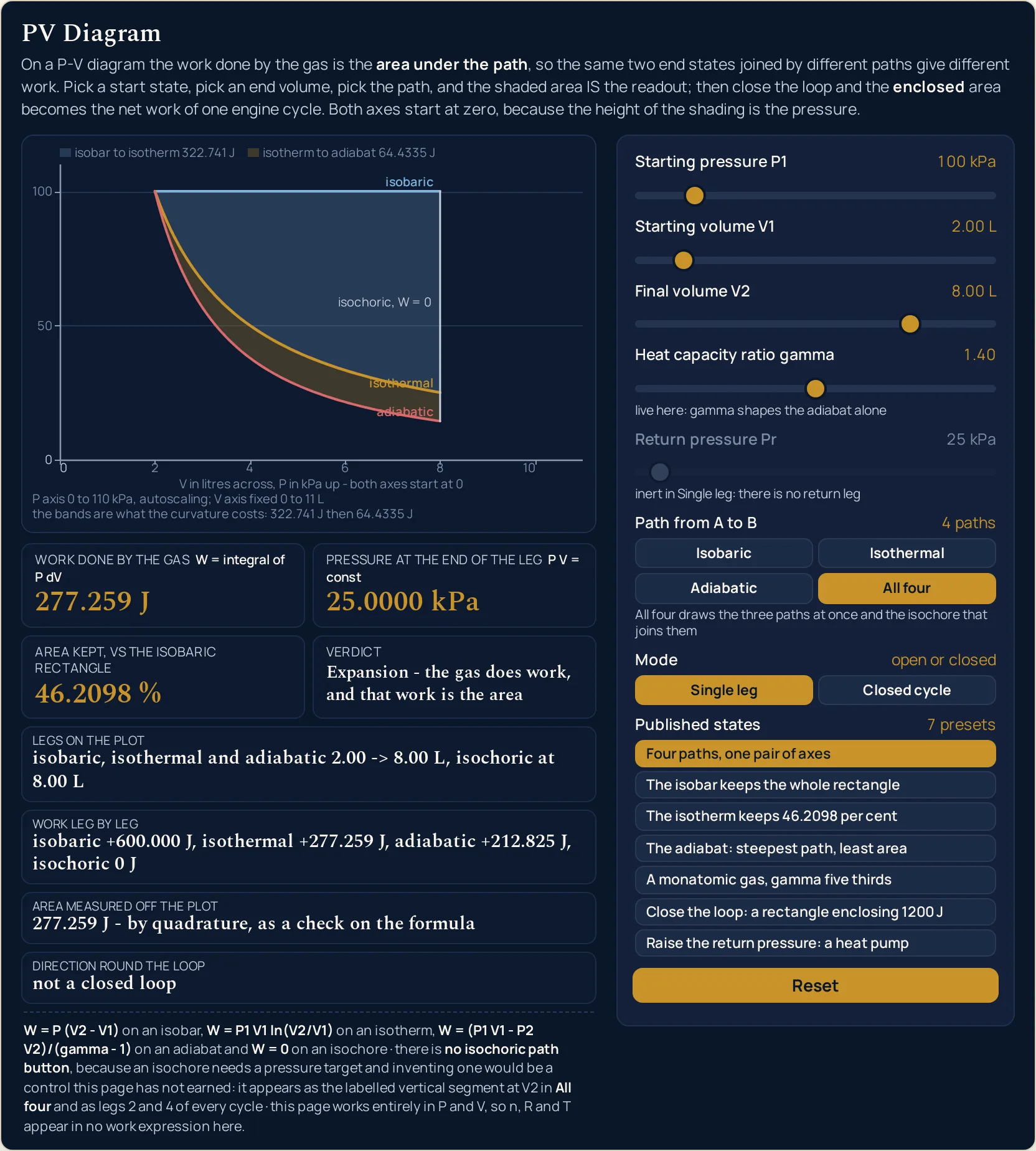
Eight readouts answer. Four cards give Work done by the gas, Pressure at the end of the leg, a third card that changes its own label with the mode, and a Verdict; a compact grid under the plot adds Legs on the plot, Work leg by leg, Area measured off the plot and Direction round the loop. On the opening state they read 277.259 J, 25.0000 kPa, 46.2098 %, Expansion - the gas does work, and that work is the area and 277.259 J - by quadrature, as a check on the formula.
That quadrature row is the lab checking itself in public. The work card comes from a closed form and the area row comes from a 401-point sum over the plotted points, so the two agree only if the shading really is the integral — and the row says so in its own words rather than leaving you to trust it. The third card is a genuinely different function again: in single-leg mode it is labelled Area kept, vs the isobaric rectangle and in cycle mode Return leg costs, of the forward output, and it prints a bare - when the two volumes are equal, because nothing can be a fraction of a rectangle of no area.
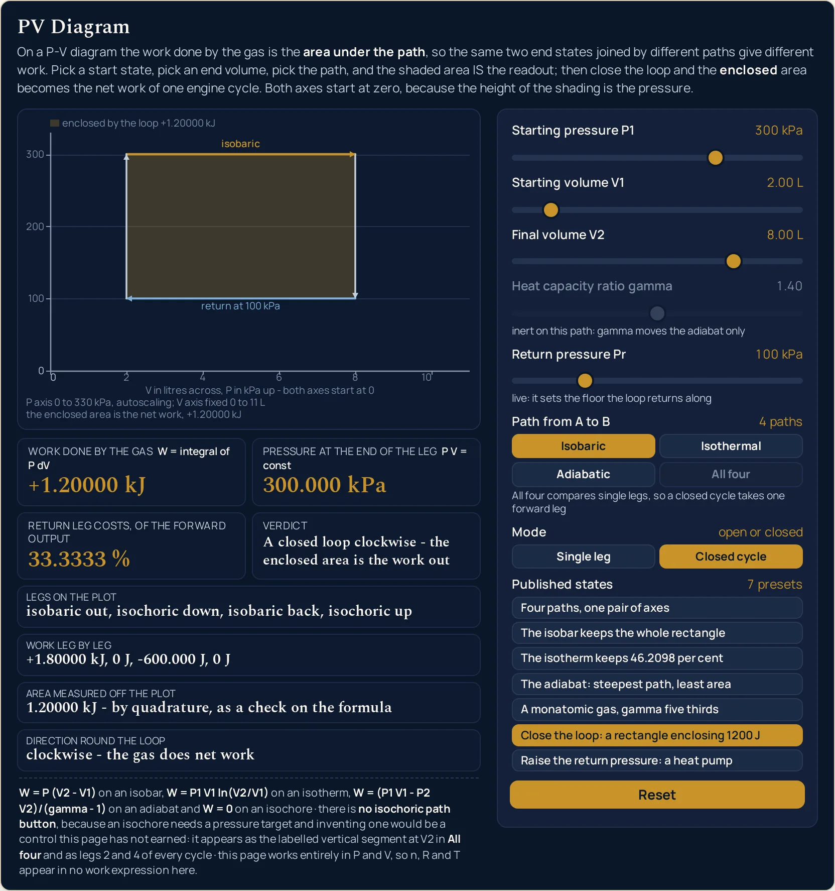
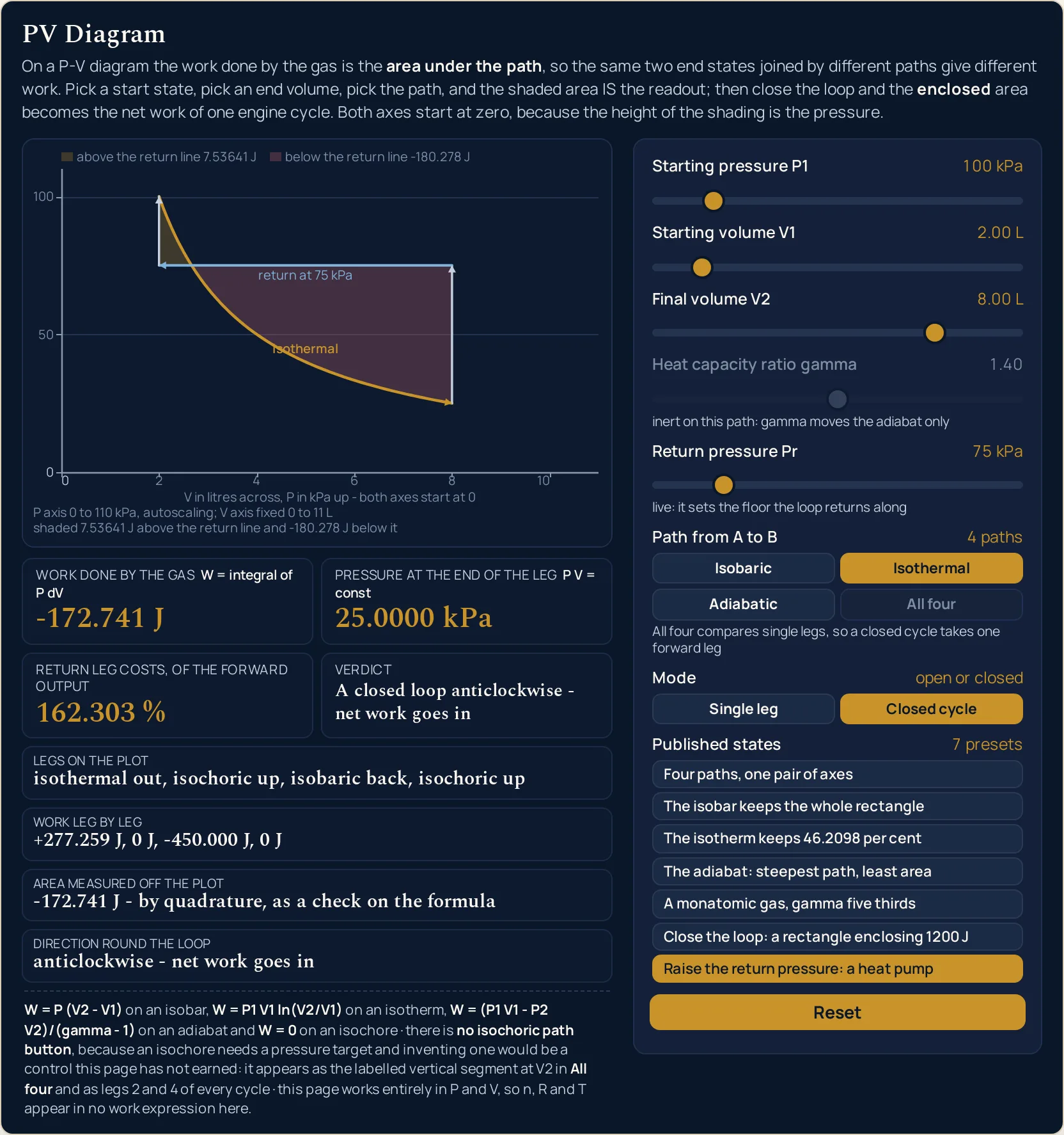
Press Close the loop: a rectangle enclosing 1200 J and the four legs read +1.80000 kJ, 0 J, -600.000 J, 0 J with the loop running clockwise - the gas does net work; press Raise the return pressure: a heat pump and the same forward leg runs anticlockwise - net work goes in for a net -172.741 J. One slider turns an engine into a refrigerator, and the sign of the net work is the direction round the loop.
What the plot refuses to draw, it says. A state with no volume change, and a return leg that simply retraces the forward one, both shade nothing at all and print No volume change - no area, so no work or Not a loop - the return leg retraces the forward leg instead of an invented area. There is no temperature axis, no entropy axis, no second scale and no piston picture anywhere on it, and nothing here computes a heat, an efficiency or an entropy change: a pressure-volume plot fixes the net work of a loop but not the heat taken into it.
| Control | Range | Step and default |
|---|---|---|
| Starting pressure P1 | 50 to 400 kPa | step 5; opens at 100 |
| Volumes V1, V2 | 1.0 to 10.0 L | step 0.1 each; open at 2.0 and 8.0 |
| Heat capacity ratio gamma | 1.10 to 1.70 | step 0.01; opens at 1.40; one preset pins five thirds |
| Return pressure Pr | 10 to 390 kPa | step 5; opens at 25; inert in single-leg mode |
| Buttons | four paths, two modes, seven presets | one press each, plus a Reset that restores every default |
How to use the PV diagram simulator
- Three paths are already on the plot when the page loads, so the first thing to do is read, not click. Four cards are answering before you have touched anything: Work done by the gas 277.259 J, Pressure at the end of the leg 25.0000 kPa, Area kept, vs the isobaric rectangle 46.2098 %, and a Verdict of Expansion - the gas does work, and that work is the area. Those four cards read one path rather than all three: in All four they report the isotherm, the middle of the fan, while the compact grid underneath carries all three paths side by side.
- Find those figures in the picture before you touch a control. Three curves leave the same point at 2.00 L and arrive at the same 8.00 L, and the two bands between them are shaded and costed in the legend: isobar to isotherm 322.741 J and isotherm to adiabat 64.4335 J. That is what the curvature of a path is worth, in joules, on one shared scale.
- Press Isobaric, then Isothermal, then Adiabatic, and watch one card at a time. The work card goes 600.000 J, 277.259 J, 212.825 J while the end-pressure card goes 100.000 kPa, 25.0000 kPa, 14.3587 kPa. The two columns descend in the same order, and the picture shows why: the lower the path finishes, the less there is underneath it.
- Notice which sliders switch themselves off while you do that. On the isobar and the isotherm, Heat capacity ratio gamma is disabled under the note inert on this path: gamma moves the adiabat only; it comes back live on the adiabat and in All four. The slider is greyed rather than hidden on purpose, so the panel keeps its height and nothing jumps under your hand.
- Take Starting pressure P1 up and note which card refuses to follow. Taking it from 100 kPa to 300 kPa on the isobar takes the work from 600.000 J to 1.80000 kJ, exactly three times, while Area kept, vs the isobaric rectangle sits at 100.000 % throughout. Pressure scales every area in proportion and changes none of their ratios.
- Drag Final volume V2 below Starting volume V1 and watch the signs turn over. Set the two volumes to 8.00 L and 2.00 L on the isotherm and the work card reads -1.10904 kJ, the end pressure climbs to 400.000 kPa, and the verdict changes to Compression - work is done on the gas. The legend under the plot changes with it, from area under the path, work out to area under the path, work in.
- Now press Closed cycle, and watch the fifth slider wake up. Return pressure Pr is disabled in single-leg mode under the note inert in Single leg: there is no return leg, because there is no return leg for it to set. In cycle mode its note becomes live: it sets the floor the loop returns along, and the shading moves from under the path to inside the loop. All four goes the other way and greys itself out, under the note All four compares single legs, so a closed cycle takes one forward leg.
- Drag the return pressure until the verdict flips. On the opening isotherm, 25 kPa gives +127.259 J and clockwise - the gas does net work; 75 kPa gives -172.741 J and anticlockwise - net work goes in. One slider, one sign, and the difference between an engine and a refrigerator.
- Read the compact grid under the plot as a decomposition, not as more evidence. Legs on the plot names the legs in order, Work leg by leg gives each one’s share — +1.80000 kJ, 0 J, -600.000 J, 0 J round the rectangle — and those shares add up to the card above. Direction round the loop and Area measured off the plot are the two that say something new.
- Treat the quadrature row as the lab marking its own work. Area measured off the plot reads 277.259 J - by quadrature, as a check on the formula at the opening state, and it is a sum over the plotted points rather than a formula. When it agrees with the card above it, the shading really is the integral; that agreement is the page’s claim and not an accident.
- Go back to All four whenever you want the comparison rather than one answer. It draws the three paths together with the vertical isochore that joins their end points, labelled isochoric, W = 0, and it shades the differences rather than three overlapping areas. Its note says as much: All four draws the three paths at once and the isochore that joins them.
- Reset is the way back when too many controls have moved to remember. It puts all five sliders, the path and the mode back to their opening values, and the cards return to 277.259 J and 46.2098 %. At most one preset is highlighted at a time, and touching any slider by hand drops the highlight altogether, so the button row never claims a state you have since changed.
Dragging is the right way to compare paths and a poor way to hit an exact figure. When you already have the pressure and the two volumes and simply want the rectangle solved for whichever one is missing, the PV diagram calculator takes them typed, in whatever units you have them in. For the representation itself — what a point on these axes means, why only a quasi-static path can be drawn, and the problems worked end to end — read the full guide to PV diagrams and thermodynamic cycles.
Worked example: change one thing at a time
Nothing in the three tables that follow was worked out here. Each row is a state the lab was put into on this page and then read back from, cell by cell, so the strings below are the lab’s own. The first table keeps both end states fixed and varies only the path, then only the gas, then takes the width away altogether.
| What was pressed | Work done by the gas | Pressure at the end of the leg | Area kept, vs the isobaric rectangle | Verdict |
|---|---|---|---|---|
| The isobar keeps the whole rectangle | 600.000 J | 100.000 kPa | 100.000 % | Expansion - the gas does work, and that work is the area |
| The isotherm keeps 46.2098 per cent | 277.259 J | 25.0000 kPa | 46.2098 % | Expansion - the gas does work, and that work is the area |
| The adiabat: steepest path, least area | 212.825 J | 14.3587 kPa | 35.4709 % | Expansion - the gas does work, and that work is the area |
| A monatomic gas, gamma five thirds | 180.945 J | 9.92126 kPa | 30.1575 % | Expansion - the gas does work, and that work is the area |
| No volume change at all | 0 J | 100.000 kPa | - | No volume change - no area, so no work |
Rows one to three are the whole argument of this lab, and they share every control but one. Same starting pressure, same starting volume, same final volume, and three work figures that differ by more than a factor of two. If the work depended only on where the gas started and finished, those three cells would carry the same string; they do not, and the picture above them shows the three different regions being measured.
Row four changes the gas and nothing else. Moving from a diatomic 1.40 to a monatomic five thirds takes the adiabatic work from 212.825 J to 180.945 J and the end pressure from 14.3587 kPa to 9.92126 kPa. Do the same on the isotherm and nothing moves at all, which is why the gamma slider refuses to be dragged there.
Row five is the identity row, and it is the one worth pressing yourself. With the two volumes equal there is no width to the region, so the work is exactly 0 J on all three paths at once, the area card gives up and prints a bare -, and the plot shades nothing whatever. The caption says so in the lab’s own words: V2 = V1, so there is no area at all and nothing is shaded.
The quadrature row, against the card above it
The panel answers the same question twice, by two routes that share no arithmetic, and prints both. The left-hand figure comes from a closed form; the right-hand one is a 401-point Simpson sum over the points the lab actually plotted, and it names itself a check. The isothermal case is the one to watch, because the logarithm behind it is worked out in the isothermal process guide rather than here.
| The state | Work done by the gas | Area measured off the plot |
|---|---|---|
| Isobaric, 2.00 to 8.00 L | 600.000 J | 600.000 J - by quadrature, as a check on the formula |
| Isothermal, 2.00 to 8.00 L | 277.259 J | 277.259 J - by quadrature, as a check on the formula |
| Adiabatic, 2.00 to 8.00 L | 212.825 J | 212.825 J - by quadrature, as a check on the formula |
| Adiabatic, gamma pinned at five thirds | 180.945 J | 180.945 J - by quadrature, as a check on the formula |
| Isothermal, 2.00 to 2.20 L | 19.0620 J | 19.0620 J - by quadrature, as a check on the formula |
| Adiabatic, 400 kPa, 1.00 to 10.00 L, gamma 1.10 | 822.687 J | 822.687 J - by quadrature, as a check on the formula |
Six rows, six matching pairs, and the rows were chosen to be awkward rather than flattering: a straight line, two curves, a pinned gas, a step so short every path nearly agrees, and all four sliders at an extreme at once. From the test harness rather than a card: across the twelve published single-leg states the two routes differ by at most about five parts in a thousand million, which is floating-point arithmetic and not physics.
Closing the loop
Press Closed cycle and the third card changes its own label, from Area kept, vs the isobaric rectangle to Return leg costs, of the forward output. That is not the same number wearing a new name: in single-leg mode it compares your path with a rectangle, and round a loop it compares what you pay on the way back with what you earned on the way out.
| What was pressed or dialled | Return pressure | Work done by the gas | Return leg costs, of the forward output | Direction round the loop |
|---|---|---|---|---|
| Close the loop: a rectangle enclosing 1200 J | 100 kPa | +1.20000 kJ | 33.3333 % | clockwise - the gas does net work |
| The opening isotherm, closed into a loop | 25 kPa | +127.259 J | 54.1011 % | clockwise - the gas does net work |
| Isothermal, 300 kPa, 2.00 to 6.00 L, return at 100 | 100 kPa | +259.167 J | 60.6826 % | clockwise - the gas does net work |
| Raise the return pressure: a heat pump | 75 kPa | -172.741 J | 162.303 % | anticlockwise - net work goes in |
The first row is the only cycle on this panel whose area is plain arithmetic. A rectangle 200 kPa tall and 6.00 L wide encloses 1200 J, and the card agrees to six figures: +1.20000 kJ. Its legs read +1.80000 kJ, 0 J, -600.000 J, 0 J, so a third of what the gas does on the way out is spent getting back, which is exactly the 33.3333 % in the fourth column.
Rows two and four share a forward leg and disagree about everything else. Both run the same isotherm out from 2.00 L to 8.00 L for +277.259 J; one comes back at 25 kPa and nets +127.259 J, the other at 75 kPa and nets -172.741 J. The return pressure alone decides whether the machine is an engine or a heat pump, and the first law guide is where that net work becomes an energy balance.
The heat pump’s leg list is the one that breaks the pattern, so read it rather than assuming it. It reads isothermal out, isochoric up, isobaric back, isochoric up — up twice, because a return pressure of 75 kPa sits above the 25.0000 kPa the forward leg finished at. Its leg works are +277.259 J, 0 J, -450.000 J, 0 J, so the return stroke alone costs more than the forward one earns. The other cycles read down on their first vertical leg, and a reader who pattern-matched them would get this one wrong.
Formula and symbol reference
The lab prints its four closed forms on itself, in a fixed line under the plot: the work is P (V2 - V1) along an isobar, P1 V1 ln(V2/V1) along an isotherm, (P1 V1 - P2 V2)/(gamma - 1) along an adiabat and 0 along an isochore. The first card carries the general statement over it, W = integral of P dV, which the four below are the closed forms of.
Not one of them mentions an amount of gas or a temperature, and that is deliberate: a pressure-volume plot has no temperature axis to read one off. The isothermal area equals the familiar nRT ln(V2/V1) only because nRT happens to equal P1 V1 on an isotherm — one clause, and the derivation belongs elsewhere. If the figures you have are an amount of gas and a temperature rather than a starting pressure, the isothermal process calculator is the one that takes them in those terms.
The relations the three curves obey as gas laws, rather than as paths to measure, are set out in the guide to the gas laws. This panel never states one: it draws the curve, shades what is under it, and leaves the law to the page that owns it.
Eleven rows follow, and only five of them are things you choose. The end pressure is wherever the path you picked happened to arrive, the volume ratio has no control at all, and the bottom three rows are readouts rather than inputs. For the five sliders the right-hand column gives the end stops and the step; for everything else it gives the strings the lab prints and the range it prints them over.
| Symbol | Meaning | SI unit | In this lab |
|---|---|---|---|
| W | Work done by the gas — the area under the path, and the first card. In closed-cycle mode the same card prints the net work of the whole loop instead, signed | joule | six significant figures, in joules below a thousand and in kilojoules at or above it: “0 J”, “19.0620 J”, “277.259 J”, “600.000 J”, “-1.10904 kJ”, “-1.48220 kJ”, “1.80000 kJ”. Round a loop it reads “+1.20000 kJ”, “+127.259 J” or “-172.741 J”. |
| P1 | Starting pressure, and what the first slider sets. It scales every area on the plot in proportion and changes none of their ratios | pascal, set in kilopascals | 50 to 400 kPa in steps of 5, echoed beside the slider as “100 kPa”, “300 kPa”, “400 kPa”. Every preset pressure is already on that grid, so a hand-drag reaches each of them exactly. |
| V1 | Starting volume, and what the second slider sets. With V2 it fixes the width of the region being shaded | cubic metre, set in litres | 1.0 to 10.0 L in steps of 0.1, echoed as “1.00 L”, “2.00 L”, “8.00 L”, “10.00 L”. Its floor of 1.0 L is what keeps the isotherm and the adiabat away from the divergence at zero volume. |
| V2 | Final volume, and what the third slider sets. It is the only control that can change the sign of the work | cubic metre, set in litres | the same 1.0 to 10.0 L in steps of 0.1, echoed as “2.20 L”, “6.00 L”, “8.00 L”. Put it below V1 and every work figure on the panel goes negative; put it exactly on V1 and they all go to zero. |
| P2 | Pressure at the end of the leg, on the second card. There is no control for it — it is wherever the path you chose has arrived | pascal | six significant figures in kilopascals, and a different function of the controls on every path: “100.000 kPa” along the isobar at any volume at all, then “25.0000 kPa”, “14.3587 kPa” and “9.92126 kPa” on the curved ones. Compressions take it the other way, to “400.000 kPa” and “696.440 kPa”. |
| gamma | Heat capacity ratio, and what the fourth slider sets. It belongs to the gas rather than to the leg, and it moves the adiabat alone | dimensionless | 1.10 to 1.70 in steps of 0.01, echoed as “1.10”, “1.40”, “1.67”. This is the one slider with a pin: five thirds is not on its grid, so the monatomic preset pins the exact value and the echo reads “1.66667”. Disabled off the adiabat, under its own note. |
| Pr | Return pressure, and what the fifth slider sets. It is the floor a closed cycle comes back along, and the one control that flips an engine into a heat pump | pascal, set in kilopascals | 10 to 390 kPa in steps of 5, echoed as “25 kPa”, “75 kPa”, “100 kPa”. Disabled in single-leg mode, under the note inert in Single leg: there is no return leg, because there is no return leg for it to set. |
| r | The volume ratio, V2 divided by V1. It has no slider and no card of its own, but it is what the third card answers to on a curved path | dimensionless | not a readout. The isothermal area fraction is ln(r)/(r - 1), which depends on r and on nothing else — which is why that card does not move at all when you drag gamma on an isotherm, while the adiabatic one moves by more than two points. |
| the area fraction | The third card, whose label changes with the mode: Area kept, vs the isobaric rectangle in single-leg mode and Return leg costs, of the forward output round a loop |
per cent | six significant figures: “100.000 %” along the isobar for every ratio and every gamma, then “46.2098 %”, “35.4709 %”, “30.1575 %”, and “184.839 %” or “247.034 %” on a compression. A bare “-” when the two volumes are equal. |
| the quadrature | The Area measured off the plot row in the compact grid — a 401-point Simpson sum over the points actually plotted, printed as a check on the card above it |
joule | the same formatter, then the lab’s own words: “600.000 J - by quadrature, as a check on the formula”, “19.0620 J - by quadrature, as a check on the formula”, “-1.10904 kJ - by quadrature, as a check on the formula”. |
| the legs | The Legs on the plot and Work leg by leg rows, which name what is drawn and price each piece of it rather than adding evidence to the first card |
joule, after a list of path names | they sum to the work card on a single leg and round a cycle; in All four the row is the three paths side by side instead. “isothermal 2.00 -> 8.00 L” with “+277.259 J” on a single leg; “isobaric out, isochoric down, isobaric back, isochoric up” with “+1.80000 kJ, 0 J, -600.000 J, 0 J” round the rectangle. |
If you read only one row twice, make it the volume ratio: it is what keeps the third card from being a restatement of the first two. The isothermal fraction depends on the ratio alone, the adiabatic one on the ratio and the gas, and the isobaric one on neither: it is 100.000 % for every setting of every slider, which no other card on the panel manages.
The physics: work is the area under the path
The claim is geometric before it is thermodynamic. Pressure is on the vertical axis and volume on the horizontal one, so a thin vertical sliver under the path is a pressure times a volume change, which is an energy; adding the slivers from one volume to the other is what taking the area means. That is why both axes on this plot begin at zero, and why the one with the shading on it could not be allowed to start anywhere else.
The consequence is the part most people have to see rather than be told. Three paths from 2.00 L to 8.00 L at 100 kPa enclose 600.000 J, 277.259 J and 212.825 J, so the same two end states give three different answers, and the difference is not small. The work is a property of the journey, never of the endpoints.
The ordering is the other half of it, and the panel asserts it rather than illustrating it. The three end pressures descend as 100.000 kPa, 25.0000 kPa, 14.3587 kPa — in the opposite order to the areas. A steeper path drops away from the starting pressure faster, so there is less left underneath it; that the adiabat is the steepest of the three is something to watch here, and the one-isotherm lab is where a single curved path gets a panel to itself.
The sign is a convention and the lab states it plainly. W is the work done by the gas, so an expansion is positive and a compression negative, and the verdict strings say which you are looking at. Run the isotherm backwards and the card goes from +277.259 J to -1.10904 kJ — not a sign flip of the same magnitude, because the gas is being squeezed through a quite different pressure range on the way back.
Round a closed loop the internal energy comes back to where it started, so the net work equals the net heat. That is an identity rather than a measurement, and it is the reason this panel carries no heat card: the loop fixes the net, and nothing on a pressure-volume plot fixes the heat going in on its own. The first law of thermodynamics guide is where that balance is set out properly.
The direction round the loop is the engine question, and it has exactly one reading. A clockwise traverse expands along the higher-pressure path and comes back along the lower one, so it earns more than it spends and the card is positive; anticlockwise is the same legs with the arithmetic reversed. The panel puts that in two fixed strings, clockwise - the gas does net work and anticlockwise - net work goes in, and never infers a direction from anything but the sign.
There is one correspondence on this panel that is stated rather than hidden. The return pressure at which the opening isotherm encloses nothing is 46.2098 kPa, and the single-leg area card at the same state reads 46.2098 %. Those are the same digits because the mean pressure of a path, as a fraction of the starting pressure, is that fraction — one fact in two forms, not two pieces of evidence.
The curve the isotherm follows is a gas law in its own right, and this panel treats it as given. It draws the path, costs the area under it, and leaves the relation between pressure and volume at fixed temperature to the guide to Boyle’s law, where it is a statement about a gas rather than a shape to integrate. The adiabat is the one curve on this plot whose shape answers to a slider.
Finally, the isochore. It is the only one of the four legs with no path button, because a vertical segment needs a pressure to aim at and inventing one would be a control this panel has not earned. It appears instead as the labelled segment at the final volume in All four, always with W = 0 written on it, and as legs two and four of every closed cycle, where its contribution to Work leg by leg is the bare 0 J.
Where the PV diagram simulator breaks down
There is no failure mode here in the usual sense. Five numbers go in, four closed forms are evaluated, and the results are drawn and printed; the interesting limits are all at the edges of that bargain. Below are the ones worth knowing about: the questions a pressure-volume plot cannot answer at all, two published states the sliders are unable to land on, and the cases where the honest thing to shade is nothing.
- A pressure-volume plot does not determine an efficiency, so this one does not compute one
- The enclosed area of a loop is the net work, and that is all it is. Working out how good an engine is needs the heat taken in as well, which no pressure-volume plot fixes on its own, so there is no efficiency card here, no coefficient of performance and no heat readout to build one from. The guide to Carnot efficiency is where the ceiling those ratios are measured against is set out, and the cycle behind it is drawn there rather than here.
- Only a quasi-static path can be drawn at all, so every curve here is an idealisation
- A line on these axes assumes the gas has one pressure and one volume at every instant of the journey, which only holds if it is taken slowly enough to stay in equilibrium throughout. Pressure-volume work performed slowly enough can be made to approach that reversible ideal; a real fast stroke cannot be drawn as a single curve at all, because there is no single pressure to plot. Nothing on this panel is animated as a real process for that reason.
- The gamma slider cannot land on the monatomic value its own preset publishes
- It steps in hundredths, so its grid runs 1.66, 1.67 and never reaches five thirds. The preset therefore pins the exact value and leaves the thumb at the nearest step, and the gap is material rather than cosmetic: pinned, the cards read 180.945 J, 9.92126 kPa and 30.1575 %; at the thumb’s own 1.67 they read 180.591 J, 9.87552 kPa and 30.0985 %. Read the cards, never the thumb.
- One published cycle is not reachable from the sliders either, and this page says which
- The adiabatic loop that collapses to three legs needs a return pressure of 14.3587 kPa, and the return-pressure slider steps in fives, so the nearest it comes is 15. The collapsed state nets +126.673 J with a return leg costing 40.4803 %, and no amount of dragging will produce it. What the slider does reach, at 15 kPa, is a near neighbour and a different cycle: +122.825 J, a cost of 42.2882 %, and a fourth leg that has not quite vanished — the caption still reports -0.0798004 J shaded below the return line.
- The zero-area verdict is reachable on one path only
- For the opening isotherm, the return pressure that encloses nothing is 46.2098 kPa, which is off a slider that steps in fives: at 45 kPa the card reads +7.25887 J and at 50 kPa it reads -22.7411 J, so the thumb steps straight over the sign change. The one state this panel does reach with no enclosed area is the isobaric retrace, where the return leg runs back along the forward leg at the same pressure, the direction row reads zero enclosed area - the return leg retraces the forward leg, and the caption reads the return leg retraces the forward leg, so nothing is enclosed.
- Degenerate states are drawn as nothing rather than as something small
- With the two volumes equal, the work is exactly zero on all four legs, the area card prints a bare -, and the plot shades no region at all under the caption V2 = V1, so there is no area at all and nothing is shaded. The retracing loop behaves the same way, with its own caption. A lab that drew a hairline sliver there would be inventing an area, which is the one thing a plot whose whole claim is the area must not do.
- Over a short enough step every path nearly agrees, which is a trap rather than a result
- Take the final volume from 2.00 L to only 2.20 L and the isotherm keeps 95.3102 % of the rectangle, ending at 90.9091 kPa rather than falling away. From the test harness rather than a card: the adiabat at the same step keeps 93.5162 %, so all three paths stay above 93 % and the three work figures are hard to tell apart. Over a short enough interval every curve is flat; that is a statement about the step, not about the paths.
- The vertical scale moves and the horizontal one does not, and the caption says so every frame
- Volume is fixed from zero to eleven litres so the width of a region never changes under you, but pressure autoscales to whatever states are in play. The caption line therefore reads P axis 0 to 110 kPa, autoscaling; V axis fixed 0 to 11 L at the opening state and P axis 0 to 330 kPa, autoscaling; V axis fixed 0 to 11 L on the rectangle. Two shaded regions of the same size on screen can be worth very different numbers of joules for that reason.
- Nothing here is a real gas, and nothing here is an engine
- The four relations the lab prints on itself are the ideal cases, with no friction, no turbulence, no leakage past a piston, no heat lost through a cylinder wall and no intermolecular forces anywhere in them. No engine, manufacturer, working fluid or fuel is named on this panel, and no cycle on it is claimed to be any particular machine. Treat a figure from here as the geometry a real design is measured against rather than as a prediction about one.
- If the horizontal axis were specific volume, the area would be work per unit mass
- Some texts plot volume per unit mass along the bottom rather than volume, and the area under the path is then the work per unit mass of the working fluid instead of the work. This lab plots volume, in litres, with the slider ranges to match, so every joule it prints is a joule and not a joule per kilogram. It is worth checking which convention a diagram uses before comparing its numbers with these.
- Two engines were compared readout by readout, and Safari was never run at all
- This cluster’s cross-browser gate put 204 readouts side by side in Chrome and in Firefox at each of four viewport widths, and found no disagreement anywhere; the two engines also landed within a pixel of each other on the panel’s height. There is a hole in that, and it is Safari: the WebKit build on this box refuses to start without privileges the harness does not hold, so Safari was never run here and nothing on this page is evidence about it. If your browser ever prints a figure this page does not, trust the panel in front of you and tell us.
Where the PV diagram simulator is actually used
- Settling the path-dependence argument in three button presses
- This is the misconception the lab exists for. Press The isobar keeps the whole rectangle, then The isotherm keeps 46.2098 per cent, then The adiabat: steepest path, least area: the starting state and the final volume never move, and the work card goes 600.000 J, 277.259 J, 212.825 J. Three presses, ten seconds, and a sentence that is hard to believe becomes a picture that is hard to argue with.
- Reading an indicator diagram, which is what this plot originally was
- Pressure-volume diagrams began as indicator diagrams, eighteenth-century tools for understanding the efficiency of steam engines; the diagram was developed in 1796 by James Watt and his employee John Southern. What it recorded was the closed loop of one stroke, and what the enclosed area gave was the work of that stroke. Pressing Close the loop: a rectangle enclosing 1200 J is as close as a browser gets to the original use of the picture.
- Showing an engine and a refrigerator as the same drawing run two ways
- Clockwise and anticlockwise are not a presentational detail on these axes: they are the power cycle and the heat pump cycle respectively. Press The opening isotherm, closed into a loop and then Raise the return pressure: a heat pump, and one slider takes the panel from +127.259 J to -172.741 J, with the direction row changing to match. Household heat pumps and refrigerators are modelled on exactly that reversal.
- Costing a return stroke before arguing about anything else
- The fourth card in cycle mode reads Return leg costs, of the forward output, and it is the figure most arguments about engines actually turn on. The rectangle spends 33.3333 % of its forward work getting back; the default isotherm loop spends 54.1011 %; the heat pump spends 162.303 %, which is why its net is negative. One card, three machines, and the reason the third is not an engine.
- Checking a textbook figure, or your own, against two independent routes
- Set the state you have been given, read the work card, then read Area measured off the plot underneath it. One is a formula and the other is a sum over the plotted points, so a figure that survives both is unlikely to be a slip. It is also the quickest way to find out whether a quoted answer assumed a path you did not.
- Seeing what the choice of gas is worth, and what it is not worth
- Press The adiabat: steepest path, least area and then A monatomic gas, gamma five thirds: the work falls from 212.825 J to 180.945 J. Now do the same on the isotherm and watch nothing happen at all — the slider will not even move. Which quantities a gas property is allowed to touch is a surprisingly common exam slip, and the disabled slider answers it without a word.
- Finding out, by pressing it, that an isochore really does zero work
- Press No volume change at all and every figure on the panel goes to zero at once: 0 J on the card, isobaric 0 J, isothermal 0 J, adiabatic 0 J, isochoric 0 J in the grid, and nothing shaded on the plot. Pressure and temperature may be doing a great deal along such a leg; the work is exactly zero rather than merely small, and no pressure is large enough to change that.
- Reading a cardiac loop without borrowing the engine sign rule
- Pressure-volume loops are used in cardiovascular and respiratory physiology as well as in thermodynamics, and the cardiac one is roughly rectangular and runs anti-clockwise. That is a different system with its own conventions, and nothing on this panel should be carried across to it unexamined — the anticlockwise string here is about a gas cycle consuming net work, which is not the claim a cardiac loop is making. Worth knowing before the same shape is met in another course.
Where to go next
A panel can show you what a choice of path costs, and that is the end of what a panel is for. PV Diagrams and Thermodynamic Cycles is where the subject itself is written out: what a point and a path on these axes mean, why the area is the work, the four legs set against each other, the closed cycle and the sign convention, and the problems worked through from their own figures. The calculator that solves the flat-topped case for any one of its four quantities heads the list of related tools below.
Three neighbouring subjects are deliberately left off this panel, and each is written up on its own terms. The first law of thermodynamics guide is where the work an area measures meets the heat and the internal energy, the guide to Carnot efficiency is the ceiling every closed cycle is judged against, and the guide to the gas laws is where the relations these curves obey are stated as laws rather than drawn as shapes.
Further out, the isothermal process guide is where the logarithm on the curved path is worked, the guide to the kinetic theory of gases is where the pressure on this axis comes from in the first place, the guide to entropy is the other state function a cycle returns to, and the guide to the laws of thermodynamics names all four in one place. Beyond thermodynamics there is the whole simulation library to work through, an index of calculators for when typing beats dragging, and the blog for everything written out at length.
Frequently asked questions
Why does the third card change its own label when I switch to Closed cycle?
Because it stops being the same measurement. In Single leg it reads Area kept, vs the isobaric rectangle and compares your path with the flat-topped rectangle over the same two volumes. In Closed cycle it reads Return leg costs, of the forward output and compares the leg you pay with the leg you earn. Letting one number keep one label across both would have been the dishonest option.
Why is the heat capacity ratio slider greyed out on the isobar and the isotherm?
Because it genuinely cannot change those answers, and the panel would rather say so than let you drag a control that does nothing. The note under it reads inert on this path: gamma moves the adiabat only. It is disabled rather than hidden so the panel does not change height under you. Pick Adiabatic or All four and it comes back live.
The monatomic preset says gamma five thirds, but the slider reads 1.67. Which does the lab use?
Five thirds exactly. That slider steps in hundredths, so its grid runs 1.66, 1.67 and never lands on 1.6666 and onwards; the preset pins the exact value and leaves the thumb at the nearest step. The echo beside it gives the pinned figure as 1.66667. Touch the slider and the pin drops: the work card falls from 180.945 J to 180.591 J.
What is the Area measured off the plot row for, if it prints the same figure as the work card?
That the two agree is the whole claim, not a redundancy. The work card comes from a closed form and that row comes from a 401-point sum over the plotted points, so they are two independent routes to one number, and the row names itself a check in its own words. If the shading were not the integral, they would part company.
Why does the area card print a hyphen instead of a number?
Because you have set the two volumes equal, and nothing can be a fraction of a rectangle that has no area. The work card reads 0 J, the verdict reads No volume change - no area, so no work, and the plot shades nothing at all rather than drawing a sliver that is not there. Move either volume slider and the figure comes straight back.
Where is the isochoric button? There are only four paths and none of them is a constant volume.
There is deliberately no isochoric path button. An isochore needs a pressure to aim at, and inventing one would be a control this panel has not earned. It appears instead in two honest places: as the labelled vertical segment at the final volume in All four, and as legs two and four of every closed cycle, always stated with its zero work.
Why does the work card sometimes read joules and sometimes kilojoules?
One formatter serves every energy on the panel and it switches at a thousand joules, on the rounded figure rather than the raw one. Below that you get six significant figures in joules, as in 277.259 J and 600.000 J; at or above it the same six figures in kilojoules, as in 1.80000 kJ and -1.10904 kJ. It is a reading convention, and the sign survives it.
Can I dial in the return pressure that makes the loop enclose nothing?
Not on a curved path. For the opening isotherm that pressure is 46.2098 kPa, and the return-pressure slider steps in fives, so the thumb straddles it at 45 and 50 without ever landing on it. The one zero-area state this panel does reach is the isobaric retrace, where the return leg runs back along the forward leg at the same pressure.
References & formula source
- Every figure on this panel comes out of five slider positions and four closed forms, and nothing is fitted. The lab prints all four on itself, in a fixed line under the plot: the work is P times the change in volume along an isobar, P1 V1 ln(V2/V1) along an isotherm, (P1 V1 - P2 V2)/(gamma - 1) along an adiabat, and exactly zero along an isochore. There is no amount of gas and no temperature anywhere in them, which is the honest form for a diagram that carries no temperature axis.
- The definition of a pressure-volume diagram, the claim that the net work of a cycle is the area enclosed by the loop, and the piece of history this page quotes all come from the Wikipedia article on the pressure-volume diagram, retrieved for this cluster on 2026-10-16. That article is the source for the indicator diagram having been developed in 1796 by James Watt and his employee John Southern, for the specific-volume caveat, and for the cardiac loop running anti-clockwise. Nothing beyond its own wording is added about any of them.
- The direction rule is the claim this page most needs attributed, and it comes from the Wikipedia article on the thermodynamic cycle, retrieved on the same date. A clockwise loop on a pressure-volume plot is a power cycle and a counterclockwise one is a heat pump cycle; a clockwise traverse makes the net work positive and the machine a heat engine, and a counterclockwise one makes it negative and the machine a heat pump or a refrigerator. The panel states the same thing in its own two direction strings.
- The quasi-static caveat comes from the Wikipedia article on work in thermodynamics, retrieved on the same date, which says that pressure-volume work performed slowly enough can be made to approach the fictional reversible quasi-static ideal transformation. That is the whole justification for drawing a path at all, and it is why nothing on this panel is animated as a real process. The same article is the source for the name of the constant-volume case.
- This panel computes no heat, no internal energy, no entropy, no efficiency and no coefficient of performance, and there is no card for any of them. That is not an omission: a pressure-volume plot fixes the net work round a loop but does not fix the heat taken into it, so an efficiency is simply not determined by one. It also models no friction, no turbulence, no leakage and no real gas, so every path on it is the quasi-static ideal above rather than a prediction about any particular engine.
- The agreement between the work card and the quadrature row is measured rather than asserted. The sim computes the first from a closed form and the second as a 401-point Simpson sum over the points it actually plotted, and the independent reference script runs the same cross-check on every published figure. Over the twelve published single-leg states the worst relative difference between the two routes is about five parts in a thousand million, which is a statement about floating-point arithmetic rather than about the physics.
- Every readout figure quoted on this page is a string this simulation printed for the button or the slider position named beside it, read back out of the running lab in a browser rather than worked out by hand. Each is computed from the exact value and rounded once, so re-deriving one printed figure from another will not always reproduce the last digit; the handful of figures here that are harness measurements rather than cards say so in their own sentences. Where a figure here and the lab part company, believe the lab, and verify anything you rely on before quoting it.
- Further reading: Pressure–volume diagram — Wikipedia