A 0.20 m2 panel standing square across a 500 N/C field, and four cards answer at once. This electric flux simulator is a free interactive lab that draws the field in cross-section, turns the panel inside it, and prints what the slider positions imply: a flux of 100.00 N·m2/C, a projected area of 0.2000 m2, a cosine of 1.0000 and the sense outward.
Turn the panel and the reading falls, reaches an exact zero edge on, and then goes negative — which is the field entering rather than leaving. Press Closed box and the arithmetic changes character completely: the field cancels against itself whatever you do to it, and only a charge sealed inside moves the net at all.
Electric Flux
Tilt a flat panel inside a uniform electric field and watch how much of the field gets through: Φ = E A cos θ, with θ measured from the panel's normal — the arrow at right angles to it — and never from the panel face. The flux is signed: positive while the field leaves through that normal, an exact zero when the panel turns edge on, negative once the field is entering. Switch to Closed box and the uniform field cancels face against face, so only the charge you put inside changes the net.
Load a real surface
Each button writes the sliders and, for the last two, presses the lab's own mode button first, then lets the simulation recompute everything. Every number you then see is the lab's own, and the line underneath quotes the cards back to you once they have settled.
The first four hold one panel in one field and change only the tilt, which is why the cosine card reads straight off as the fraction of the flux that survives. The last two close the surface up, and the difference between them is a single nanocoulomb.
Pick a surface above, or drag the sliders yourself.
What Is the Electric Flux Simulator?
The electric flux simulator is a free interactive physics lab that runs in your browser, with nothing to install and no sign-up. It draws a uniform electric field in cross-section as evenly spaced horizontal lines, stands a flat panel in the middle of them, and turns that panel about its centre while you watch. A gold arrow out of the panel's face is its normal, an arc is drawn between that arrow and the field, and the lines that actually cross the panel are drawn bright while the rest stay faint.
Four controls drive it, each printing its own setting beside its name. Field strength E runs 0 to 1000 N/C in steps of 10 and opens at 500, and Surface area A runs 0.02 to 0.50 m2 in steps of 0.01 and opens at 0.20. Angle from the normal runs 0 to 180° in single degrees and opens square on at 0. Enclosed charge runs -5 to +5 nC in steps of 0.1 and only appears once the surface is closed.
Four cards carry the answer. The headline is the flux itself to two decimals; under it sit the projected area and the cosine of the angle, both to four decimals and both signed, and a one-word sense. At the opening setting those read 100.00 N·m2/C, 0.2000 m2, 1.0000 and outward.
The angle is taken from the normal arrow and never from the panel face, and that one distinction is what the drawing exists to make unmissable. Set the angle to 30° and the headline reads 86.60 N·m2/C. A field quoted as 30 degrees from the surface is 60 degrees from the normal, and that setting reads 50.00 instead. The gap is 36.60, and both numbers look perfectly reasonable on their own.
Opening the panel out to its square-on reading makes the sweep read as a percentage, which is why the lab opens on these two figures: at 500 N/C through 0.20 m2 the product is exactly 100. From there 0° gives 100.00, 30° gives 86.60, 45° gives 70.71, 60° gives exactly half at 50.00, 90° gives 0.00, 120° gives -50.00 and 180° gives -100.00.
The flux keeps its sign in every reading, and the sense card says which kind of zero you are looking at. It prints outward while the flux is positive and inward once it has gone negative. A true zero has three different causes, so it gets three different words: grazing for a panel turned edge on in a real field, no field when the field slider is at 0 N/C, and balanced for a closed box whose faces cancel. The headline prints 0.00 in all three cases, and they are not the same physics.
Press Closed box and the panel becomes a box in the same field, with the charge slider appearing beside the others. The headline card relabels itself to the net flux out of the whole surface. Wind the field slider anywhere you like and that net stays at 0.00 N·m2/C while the box is empty, because as many field lines enter the box as leave it. Tilt the box as well and it still does: the six faces move to angles that pair off, and each pair cancels.
The sentence strip under the drawing shows the cancellation face by face rather than asserting it. Square on at 500 N/C with faces of 0.16 m2 it reads +80.00, -80.00 and four zeros; tilted to 30° the same box reads +69.28, -69.28, -40.00, +40.00 and two zeros. Every pair still sums to nothing.
Now move the charge slider, and the net stops being zero. One nanocoulomb inside gives 112.94 N·m2/C out of that surface, and a charge of -5 nC gives -564.70 flowing inward. That reading does not depend on the field slider, on the area slider or on the tilt: it is the enclosed charge divided by the permittivity of free space, ε0 = 8.8541878128e-12 F/m, and nothing about the surface enters it.
A compact grid under the cards repeats the three slider settings and adds the square-on flux the panel would take at 0°, which is the field times the area. In the closed mode it also shows the enclosed charge and the Gauss reading beside it. The last cell is fixed: N·m2/C = V·m. Those are two names for one unit, since a volt is a joule per coulomb and therefore a newton metre per coulomb, and the lab offers no conversion factor between them because there is none.
The drawing is honest about what it is and is not drawing. The field lines sit at a fixed spacing, so how many cross the panel follows the projected area and not the field strength; at E = 0 no line is drawn at all. The panel is a cross-section with its out-of-page width held fixed, so its drawn height really is the projected area to scale, and the closed box is drawn on that same scale. The eight arrows on the charge are a fixed count: their length carries the size of the charge and their direction carries its sign, so they can never be counted as a quantity.
What the lab leaves out, stated as omissions rather than as assumptions that happen to hold. It handles one flat surface in one uniform field; a curved surface has a normal that turns from point to point and a field that varies across the surface needs an integral, and the lab draws neither. It takes the field as a slider setting and works no field out from any charge. Nothing on the panel is a measurement: every digit is arithmetic on four slider positions, so verify any figure against your own source before you use it for anything that matters.
| Control | Range | Step, default and what it moves |
|---|---|---|
| Field strength E | 0 to 1000 N/C | steps of 10 N/C, opening on 500, where the read-back beside the slider says "500 N/C". The flux is directly proportional to it in the flat-panel mode: halve the field and every flux reading halves with it. At 0 N/C the headline is an exact 0.00 and the sense card says "no field" rather than "grazing", because an edge-on panel and an absent field are different states that happen to share a number. In the CLOSED-BOX mode this slider moves nothing at all in the net reading, which is the whole point of that mode |
| Surface area A | 0.02 to 0.50 m2 | steps of 0.01 m2, opening on 0.20, where the read-back says "0.20 m2". With the field at its default that makes the square-on flux exactly 100, so every cosine then reads straight off as a percentage. The projected-area card is this figure multiplied by the cosine, so it runs from the full 0.2000 m2 square on down to 0.0000 m2 edge on and then negative past 90 degrees. In the closed-box mode this is the area of one FACE of the box |
| Angle from the normal | 0 to 180 degrees | single-degree steps, opening on 0, where the read-back says "0 deg". This is the angle between the field and the panel's NORMAL arrow, never the angle to the panel face - read it off the face by mistake and you have entered the complement, which is a different answer. Under 90 degrees the flux is positive and the field is leaving; at exactly 90 it is an exact 0.00 and the sense card says "grazing"; past 90 it is negative and the field is entering. In the closed-box mode it tilts the whole box, and the net stays at zero at every tilt |
| Enclosed charge | -5 to +5 nC | steps of 0.1 nC, opening on 0. The slider is hidden in the flat-panel mode and appears when the box closes, because an open panel encloses nothing. It is the ONLY control that moves the net flux out of the closed box: 1.0 nC gives 112.94 N m^2/C outward and -5 nC gives -564.70 inward, whatever the field, the area and the tilt are doing. That reading is the charge divided by the permittivity of free space, 8.8541878128e-12 F/m |
| Closed box and Reset | two buttons | the first is a toggle and shows the ACTION rather than the state, so it reads "Closed box" while the flat panel is on screen and "Flat panel" once the box is. The second is labelled "Reset" and restores every default including the mode, which is why the landing page's two closed-box presets press Reset and then the mode button in that order. There is no pause or play control: the picture eases to a new tilt over about a quarter of a second and then rests, so there is no animation to stop |
How to use the electric flux formula simulator
- Read the four cards before you touch anything. They are already answering for a panel square on to the field: Electric flux
100.00 N·m2/C, Projected area0.2000 m2, Cosine of the angle1.0000and Sense through the normaloutward. The first and second carry their own relation beside the label. - Find the gold arrow before you move anything. It comes out of the panel's centre, it is labelled
normal, and the arc beside it is the angle the lab means. The caption under the drawing says so outright:theta is measured from the NORMAL arrow, not from the panel face. - Drag Angle from the normal and watch three things move together. The cosine card, the projected area card and the drawn height of the panel all fall at the same rate, because the second is the panel area multiplied by the first and the third is the second drawn to scale. At
60°they read0.5000and0.1000 m2. - Keep going past 90 degrees, which is where most of the value is. At
90°the flux card is an exact0.00 N·m2/Cand the sense card saysgrazing. One degree further and the reading is negative: at120°it is-50.00 N·m2/Cand the sense card saysinward. - Drag Field strength E and notice what does not move. The flux and the square-on grid cell scale with it, but the cosine and the projected area do not, and neither does the spacing of the drawn field lines. At
0 N/Cno line is drawn at all and the sense card readsno fieldrather thangrazing. - Drag Surface area A to separate the area from the flux. It runs
0.02to0.50 m2, the panel is redrawn to match, and both the flux and the projected area follow it in proportion. The cosine card does not move at all, because a cosine is about the tilt and nothing else. - Press Closed box, and then go back to the field slider. The panel becomes a box of the same material and the headline card relabels itself to the net flux out of the whole surface. Drag the field anywhere between
0and1000 N/Cand the net stays at0.00 N·m2/C, with the sense card readingbalanced. - Read the strip under the drawing for the reason. It prints the six faces as a sum —
+80.00, -80.00, 0.00, 0.00, 0.00 and 0.00on the preset box — so the cancellation is on screen rather than asserted. Tilt the box and the six numbers all change while the sum does not. - Now drag Enclosed charge, the one control that does move it. At
1.0 nCthe net is112.94 N·m2/Cand at-5.0 nCit is-564.70. Neither figure depends on the field, the area or the tilt, which is the whole reason the closed mode exists. - Press Reset when you have finished. It restores every default including the mode, so you always land back on the flat panel square on at
500 N/Cthrough0.20 m2, which is the state every figure on this page is measured against.
Dragging is the right way to find out which readings move together and a poor way to land on a particular state, because the angle slider alone has 181 positions. The six preset buttons above exist for that reason, and the electric flux guide is where the subject itself is argued from scratch, with the definition set out and the problems worked step by step.
One thing this panel cannot do is run the relation backwards. It only ever goes forwards, from three slider positions to a flux, so a problem that hands you a flux and asks for the area, the field or the angle needs the electric flux calculator instead, which solves in all four directions and shows the working for each.
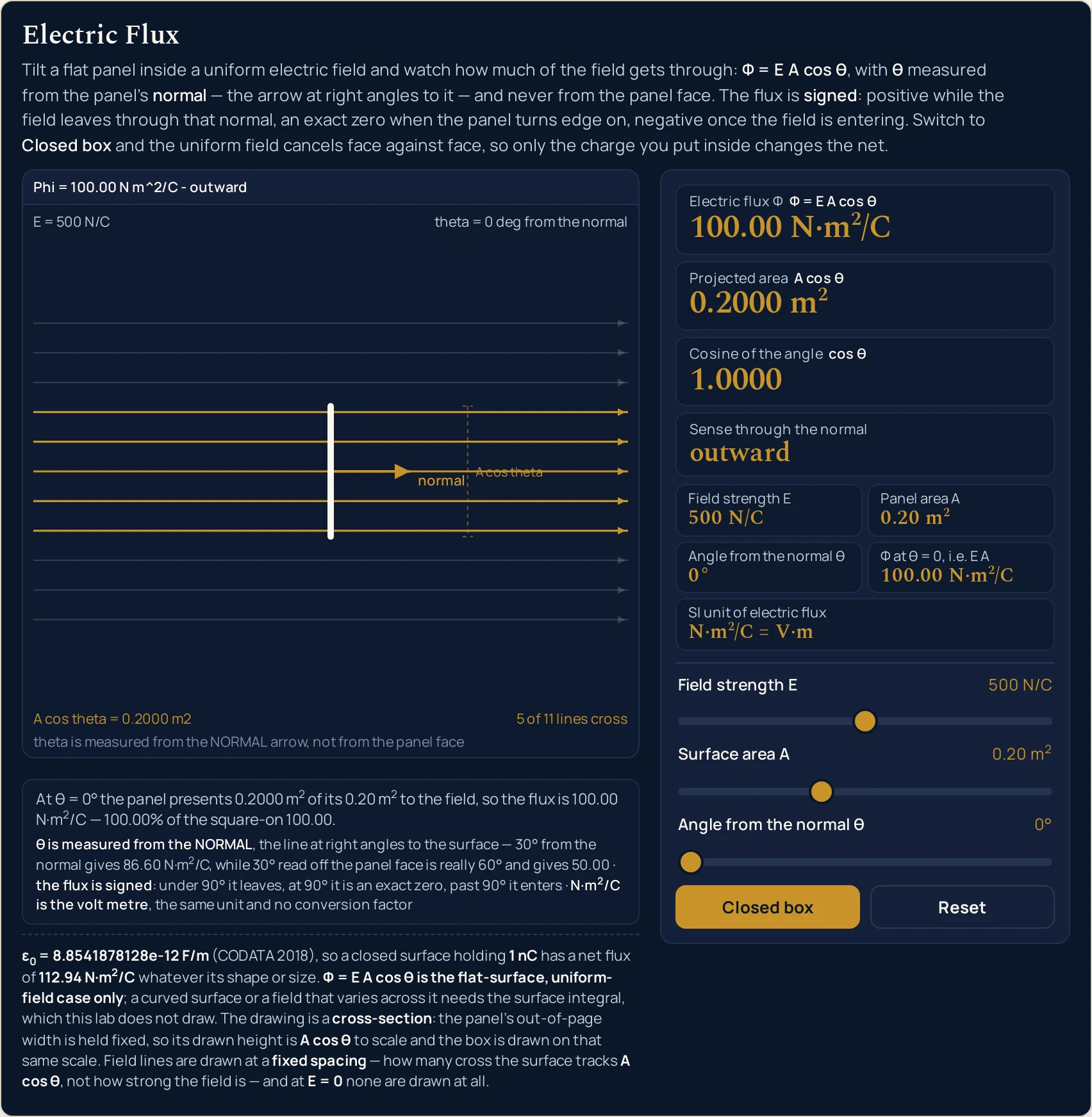
100.00 N·m2/C against a square-on maximum of the same figure, because at 0° there is no tilt to lose anything to. The band in the drawing writes the unit in ASCII, because the canvas has no markup to write a superscript with.Worked example: change one thing at a time
Nothing in the two tables below was worked out here. Each row is a state the lab was put into through its own sliders and buttons and then read back from, cell by cell, so every string in them is the panel's own. The first table moves the angle and holds the field and the area still.
One: the tilt, with the panel and the field left alone
The opening panel throughout — 500 N/C through 0.20 m2 — so the square-on flux is exactly 100.00 N·m2/C and each flux reading is also the percentage of it that survives. Read the last three rows before anything else.
| Angle from the normal | Cosine card | Projected area card | Electric flux card | Sense card | What the panel is doing |
|---|---|---|---|---|---|
| 0° | 1.0000 | 0.2000 m2 | 100.00 N·m2/C | outward | square on — every line through |
| 30° | 0.8660 | 0.1732 m2 | 86.60 N·m2/C | outward | the tilt has cost 13.40 per cent |
| 45° | 0.7071 | 0.1414 m2 | 70.71 N·m2/C | outward | the half-way angle is not the half-way flux |
| 60° | 0.5000 | 0.1000 m2 | 50.00 N·m2/C | outward | exactly half |
| 90° | 0.0000 | 0.0000 m2 | 0.00 N·m2/C | grazing | an exact zero, not a leftover |
| 120° | -0.5000 | -0.1000 m2 | -50.00 N·m2/C | inward | the mirror of 60 degrees, with the sign turned over |
| 180° | -1.0000 | -0.2000 m2 | -100.00 N·m2/C | inward | square on again, entering against the normal |
The table is symmetric about the fifth row, and that symmetry is the sign convention in one picture. Sixty degrees and 120 degrees give the same size of flux with opposite signs; so do nought and 180. Nothing about the field has changed between a pair — only which side of the panel it is arriving at.
The second row is the one to take away from this page. A field described as 30 degrees from the surface is 60 degrees from the normal, so the honest comparison is row two against row four: 86.60 against 50.00 N·m2/C. Reading the angle off the wrong line changes the answer by 36.60 and leaves a number that looks entirely reasonable.
The field strength never appears in that argument, because it cancels out of the comparison: both readings share it. What the slider does change is the scale of the whole column, and the electric field guide is where that quantity is a subject in its own right rather than an input to this one.
Two: the closed box, where the field stops mattering
Each row below is the box the last two preset buttons build, with faces of 0.16 m2. The first three move the field and the tilt and change nothing at all; the last four move the charge slider and change everything. The final column is the strip the lab prints under the drawing.
| What the box is doing | Field strength | Enclosed charge | Net flux card | Sense card | Face by face, under the drawing |
|---|---|---|---|---|---|
Empty, square on, field at 500 N/C |
500 N/C | 0.0 nC | 0.00 N·m2/C | balanced | +80.00, -80.00, 0.00, 0.00, 0.00 and 0.00 |
Empty, tilted to 30° |
500 N/C | 0.0 nC | 0.00 N·m2/C | balanced | +69.28, -69.28, -40.00, +40.00, 0.00 and 0.00 |
| Empty, field at its maximum | 1000 N/C | 0.0 nC | 0.00 N·m2/C | balanced | +160.00, -160.00, 0.00, 0.00, 0.00 and 0.00 |
| One nanocoulomb inside | 500 N/C | 1.0 nC | 112.94 N·m2/C | outward | +80.00, -80.00 and four zeros; the charge then adds 112.94 |
| The same charge with the field switched off | 0 N/C | 1.0 nC | 112.94 N·m2/C | outward | six zeros, because there is no field; the charge still adds 112.94 |
| The charge slider at its positive end | 500 N/C | 5.0 nC | 564.70 N·m2/C | outward | +80.00, -80.00 and four zeros; the charge then adds 564.70 |
| The charge slider at its negative end | 500 N/C | -5.0 nC | -564.70 N·m2/C | inward | +80.00, -80.00 and four zeros; the charge then adds -564.70 |
Three different sets of six face figures, one answer. The square-on box, the tilted box and the box at double the field all print different sums under the drawing and all land on an exact 0.00 N·m2/C. That is not a coincidence the lab is hiding: a uniform field puts exactly as much in as it takes out, whatever the box is doing.
Then one nanocoulomb changes the answer and nothing else does. Rows four and five are the same charge with the field at 500 N/C and at 0 N/C, and they print the identical 112.94 N·m2/C. The charge inside is the only thing the net has ever depended on, and the electric charge guide is where that quantity is set out properly.
Formula and symbol reference
The band at the head of this page carries two relations rather than one, because the lab has two modes and its headline card relabels itself between them. Every reading on the panel is one of those two, a factor inside one of them, or a statement about the unit they share.
The symbol column below uses the panel's own names, and the “in this lab” column gives each slider's own end stops with the labels the panel printed at those positions. Four of the rows are not controls at all: the projected area, the cosine, the square-on flux and the permittivity are computed or stated rather than set.
| Symbol | What it is | SI unit | In this lab |
|---|---|---|---|
| Φ | Electric flux: a single signed number for the whole surface, and the quantity this lab is named after. It is a scalar — the direction has already been spent in the cosine | N·m2/C, which is V·m | the headline card, two decimals. Over the states in these tables it runs from -564.70 to 564.70 N·m2/C; on the flat panel alone the widest reading the sliders reach is -500.00 N·m2/C, at 1000 N/C through 0.50 m2 turned right over. |
| E | Electric field strength at the panel, taken as given here. This lab never works one out from a charge and a distance | N/C, which is V/m | the first slider, 0 to 1000 N/C in steps of 10, opening on 500 N/C. At 0 the drawing shows no field lines at all and the sense card reads no field rather than grazing. |
| A | The true area of the flat surface, not the area facing the field. In the closed-box mode it is the area of one face of the box | m2 | the second slider, 0.02 to 0.50 m2 in steps of 0.01, opening on 0.20 m2. The two closed-box presets set it to 0.16 m2, which needs that hundredth step to land on. |
| θ | The angle between the field and the surface normal — never the angle to the surface itself, which is its complement | degree | the third slider, 0 to 180° in single degrees, opening square on at 0°. Under 90° the flux is positive, at 90° it is an exact zero, past 90° it is negative. |
| A cos θ | The projected area: the shadow the panel casts across the field, and the only part of it the flux counts. Signed, so it turns negative with the cosine | m2 | the second card, four decimals. On the opening panel it runs 0.2000, 0.1732, 0.1414, 0.1000, 0.0000 and -0.1000 m2 across the sweep table above. |
| cos θ | The cosine of that angle, which is the fraction of the square-on flux the tilt leaves behind | none — a ratio | the third card, four decimals and signed. It is snapped to an exact 1.0000, 0.0000 or -1.0000 at the multiples of 90 degrees, where the true cosine really is exactly that. |
| Qenc | The charge enclosed by the closed surface. There is no such quantity for an open panel, which is why the slider is hidden until the box closes | nanocoulomb (nC) on the slider | the fourth slider, -5 to +5 nC in steps of 0.1, opening on 0.0 nC. It is the only control that moves the net flux out of the closed box. |
| ε0 | The permittivity of free space: a constant of the vacuum, stated by the lab rather than entered | F/m | a fixed block under the panel, 8.8541878128e-12 F/m (CODATA 2018). The Gauss grid cell is the enclosed charge divided by it. |
| Φ at θ = 0 | The most this surface could ever take, square on to the field — the field multiplied by the area | N·m2/C | a grid cell. It reads 100.00 N·m2/C on the opening panel, 80.00 on the two closed-box presets, and 500.00 at the top of both the field and the area sliders. |
The last cell of the grid is fixed and says more than it looks: N·m2/C = V·m. A volt is a joule per coulomb, which is a newton metre per coulomb, so a volt metre and a newton square metre per coulomb are one unit under two names. There is no conversion factor and the lab offers none, which is also why a field in N/C and the same field in V/m drive the identical reading.
The panel takes that field as a slider setting and never works one out. If your problem starts from a charge and a distance instead, the electric field calculator produces the number you would then dial in here.
The physics: why the cosine is there
A flux counts how much field crosses a surface, so the whole area is the wrong thing to multiply by. What counts is the surface's shadow across the field, and the second card prints it: the projected area, which is the panel area multiplied by the cosine of the tilt.
The drawing makes that literal rather than symbolic. The panel is drawn in cross-section with its out-of-page width held fixed, so its drawn height is the projected area to scale. Tilt it and the shape you see shortening is the quantity on the second card, falling at exactly the rate the card does.
That is also why the angle must be taken from the normal. A shadow has to be measured against something, and the gold arrow is that something: at 0° from it the panel lies flat across the field and loses nothing. Take the angle off the panel face instead and you have its complement, which puts a sine where a cosine belongs and a plausible wrong number on your page.
The sign comes from the same choice. Picking a normal is picking which face you call the front; a field leaving through that face is positive and one entering it is negative. The sense card names which, and it is driven by the sign of the flux rather than by comparing the angle with 90 degrees, so the three different zeros can be told apart.
Closing the surface up removes the geometry from the problem altogether. Every face of a box is a flat panel with its own normal, so the lab adds them up — and a uniform field contributes exactly as much on the way in as on the way out, at every tilt. What is left is the charge inside, divided by the permittivity of free space, and the shape of the box has dropped out of the answer.
One last note on the letter. The same Greek capital stands for several unrelated quantities across physics, which is why the panel labels its headline card in words as well as in symbols, and why the physics symbols guide is worth a glance if you met it somewhere else. On this page it always means an electric flux.
| Part of the drawing | What it paints | What it does not claim |
|---|---|---|
| the headline band | The strip across the top of the drawing. On the opening panel it reads Phi = 100.00 N m^2/C - outward, and with the box closed and a charge inside it reads net Phi = 112.94 N m^2/C - outward. The canvas writes in ASCII because fillText has no markup; the cards beside it carry the real symbols |
it never drops the unit and never drops the word net. On a narrow canvas the band shortens rung by rung instead of overflowing, and at a 186 px article column it is still drawing Phi = 100.00 N m^2/C. A shortened band is a shorter claim, not a different one |
| the normal arrow and its arc | The gold arrow out of the panel's centre, labelled normal at its tip, with an arc drawn between it and the field direction. The caption under the scene reads theta is measured from the NORMAL arrow, not from the panel face |
it does not let the angle be read off the panel. That is the one mistake this topic turns on, so the line the angle is measured from is drawn, labelled and captioned rather than implied. Every rung of the caption ladder keeps the word NORMAL, down to the shortest, from the NORMAL |
| the field lines | Eleven evenly spaced horizontal lines across the whole scene, with the ones that actually cross the panel drawn bright and the rest left faint. The drawing counts them in words at the foot: 5 of 11 lines cross on the opening panel, 0 of 11 lines cross edge on |
the spacing is fixed, so a reader can never count lines as a measure of the field strength. The count follows the projected area instead, in whole lines: on the largest panel it runs 11 of 11 square on down to 0 of 11 edge on, and on the smallest it is 1 of 11 even square on. At 0 N/C no line is drawn at all |
| the panel, and the box it becomes | A flat panel drawn in cross-section with its out-of-page width held fixed, so its drawn height is the projected area to scale. Press the mode button and it becomes a closed box drawn on that same scale, so the box's front face is exactly as tall as the flat panel would be | the box is not drawn larger to look more important. One shared scale across both modes is what makes the two pictures comparable, and the longest panel is divided down so that a box turned 45 degrees still fits the scene rather than being clipped |
| the charge at the centre | Eight short arrows radiating from a dot in the middle of the closed box, pointing outward for a positive charge and inward for a negative one, with their length following the size of the charge | the number of arrows is fixed at eight, so it can never be read as a quantity. Only the length carries the size and only the direction carries the sign. There are not twice as many arrows for twice the charge, because a count on a drawing invites exactly the wrong kind of arithmetic |
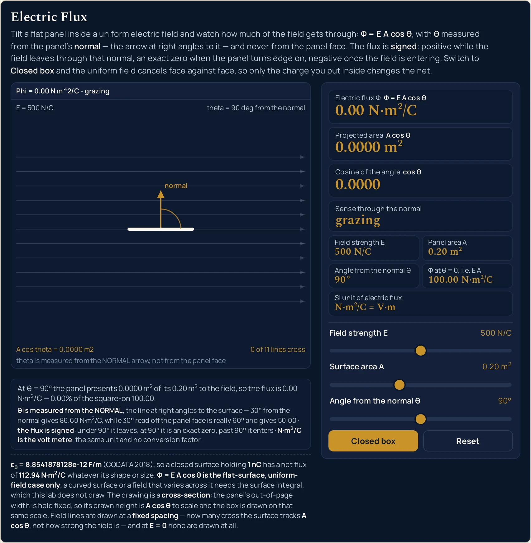
0.00 N·m2/C rather than a leftover like 3.06e-15, and the sense card says grazing — which is a different state from the same 0.00 at a field strength of zero.Where the electric flux formula breaks down
Every state the four sliders reach is answered, and the arithmetic is not where this panel can let you down. What it cannot be is a real surface in a real field, and what it refuses to do is treat its own idealisations as facts. The first two items below matter more than the rest put together.
- A field that is not uniform across the surface
- This is the hard limit, and the drawing is built on the assumption. The relation multiplies one field by one area, so it takes the same field at every point of the panel. Close to a charge, near an edge or anywhere with a gradient that is false, and the honest version is an integral over the surface that adds up a different field at every patch. This lab draws evenly spaced lines because its field really is the same everywhere, which no real field is.
- A surface that is not flat
- A curved surface has a normal that turns from point to point, so there is no single angle to put on the slider and no single cosine to multiply by. For a closed curved surface the lab's second mode still applies and needs no geometry at all, which is the point of it. For an open curved one, the only honest route is to break it into flat patches and add their fluxes.
- The field is an input here, never an output
- The first slider is where E starts, not where it comes from. Nothing on this panel works a field out from a charge and a distance, and there is no charge or radius control for the flat-panel mode. The electric field simulator is where the field of a charge is the subject, including how quickly it falls off, and it produces the kind of number this lab then takes as given.
- The box is drawn as a box, and the law does not care
- The closed mode draws a square box because something has to be drawn, but the net flux out of it is the enclosed charge divided by the permittivity and nothing else. A sphere, a cube or a crumpled bag holding the same charge gives the same
112.94 N·m2/Cfor1.0 nC. Read the drawn shape as an illustration rather than as a condition of the result. - A flux is not a field, and not a potential either
- The flux card and the field slider have different units and answer different questions: one is the field at a point, the other is a count of field crossing a whole surface. The other scalar built from the field is the electric potential, which is a third quantity again — the electric potential guide covers it, and nothing on this page computes one.
- The charge drawing is a sign and a size, not a count
- Eight arrows radiate from the charge at the centre of the box and there are always eight of them. Their length carries the size of the charge and their direction carries its sign; doubling the charge does not add arrows. A count on a drawing invites arithmetic the drawing cannot support, so the lab fixes the count and lets the length do the work.
- Four slider positions, and no measurement anywhere
- You set four controls and the lab reports what they imply. There is no box to type a measured flux into, no unit menu and no way to run the relation backwards, and the preset values are chosen to be legible rather than to describe any real apparatus. Verify any figure against your own source before you use it.
Where electric flux is actually used
- Telling the two readings of an angle apart
- This is what the panel exists for. Load Tilted 60 degrees and then set the slider to 30, and you have both readings of the same physical description on screen:
50.00and86.60 N·m2/C. The normal arrow and its arc are drawn the whole time, so the question “from which line?” is answered by the picture rather than by a footnote. - Seeing a sign convention instead of memorising one
- Drag the angle from
0°to180°in one movement and watch the flux card fall through an exact zero and come back negative, with the sense card changing word underneath it. The signed projected area does the same thing one card up. It is a far more durable memory than a rule about cosines being negative in the second quadrant. - Getting Gauss's law from a demonstration rather than a derivation
- Press Empty box - net zero and then drag the field slider from end to end. Nothing happens to the net, and the strip under the drawing shows exactly why, face by face. Press Charge in the box and the net jumps to
112.94 N·m2/C. Two buttons and one slider carry the whole statement that the enclosed charge is all that matters. - Checking an answer before checking its arithmetic
- The grid cell for the square-on flux is the ceiling for any reading at that field and area, because the cosine cannot exceed one. If a flux you have worked out is larger than it, the error is upstream of the arithmetic. On the opening panel that ceiling is
100.00 N·m2/C, and at the top of both sliders it is500.00. - Accounting for a sensor that is not quite aligned
- Anything that responds to a field through a face loses the cosine of its misalignment, and the sweep table makes the shape of that loss concrete: 30 degrees still keeps 86.60 per cent, while 60 degrees keeps only half. The cosine is forgiving near zero and brutal near 90, which is the opposite of most people's intuition about small errors.
- Setting up the contrast with the magnetic case
- The same cosine geometry appears for a different quantity on the magnetic side, and the difference is worth one sentence: electric field lines start and end on charges, magnetic ones do not, so only the electric closed-surface law has a charge term in it at all. The magnetic flux guide is where that side belongs, and this page stops here.
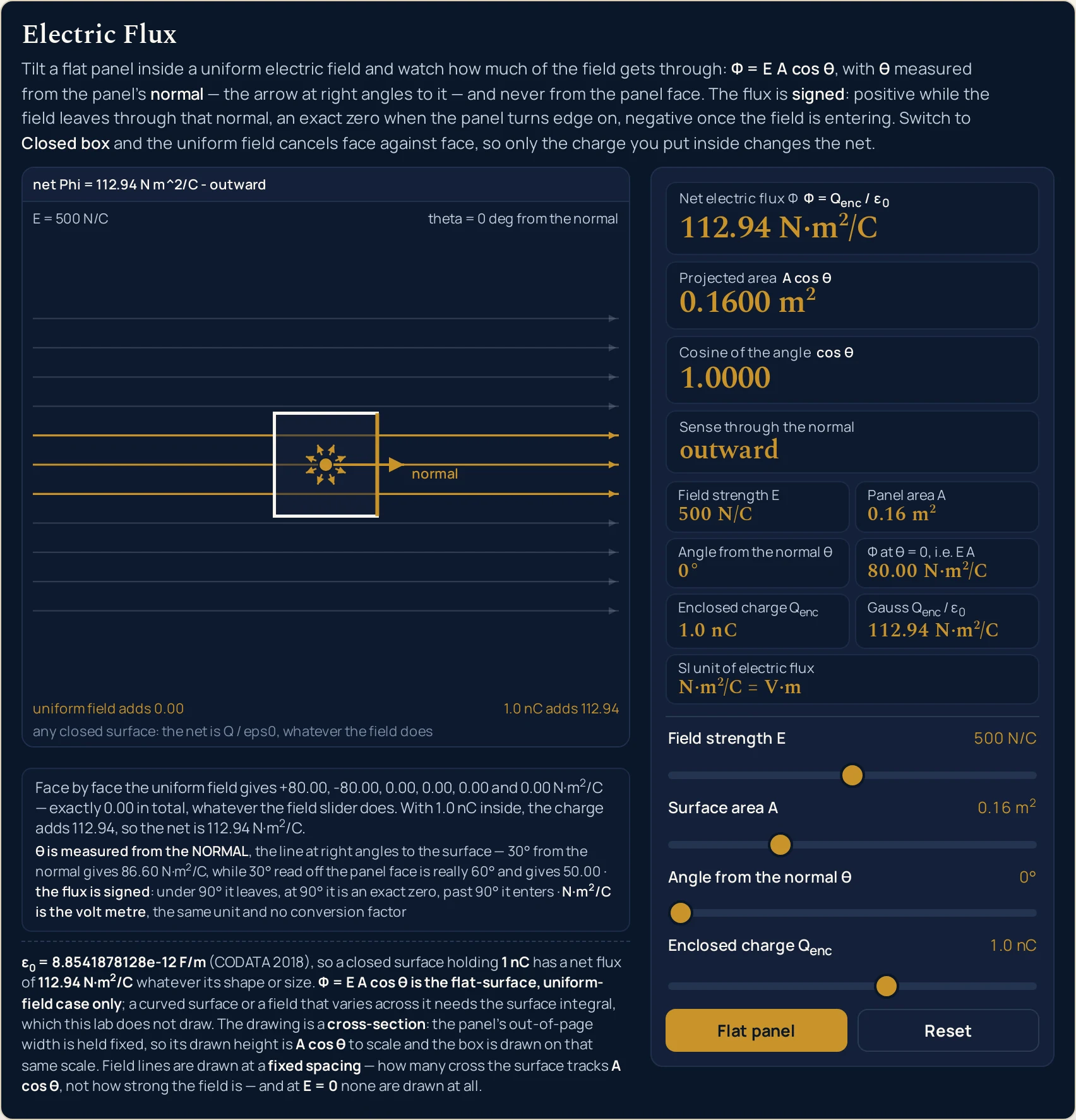
1.0 nC sealed inside. The net reads 112.94 N·m2/C, and the strip states where it came from — the uniform field adds 0.00 and the charge adds all of it. Move the field slider from end to end and that number does not change.Where to go next
A panel can put you in a state and let you move one thing at a time, and that is the end of what a panel is for. The electric flux guide is where the subject is written out: the definition, the angle trap in prose, the closed-surface law and the worked problems, with each step set out in full.
Three posts own the pieces this lab takes as given. The electric field guide covers the quantity on the first slider, the electric charge guide covers what produces it and what the box encloses, and Coulomb's law is the inverse-square relation behind the closed-surface result. The capacitance guide is where a flux between two plates starts doing something useful.
On the tool side, the electric flux calculator takes typed figures and solves in four directions, the electric field calculator produces the field this lab takes as given, and the magnetic flux calculator runs the same cosine geometry for the magnetic quantity.
Two neighbouring pictures sit beside this one: the electric field simulator and the magnetic flux simulator. Beyond them there is the simulation library, an index of calculators, and the blog for everything written out at length.
Frequently asked questions
Why does the lab insist the angle is measured from the normal?
Because reading it off the panel face instead gives a different, perfectly plausible answer. The gold arrow out of the panel is the normal, and the arc is drawn between that arrow and the field so the measured line cannot be mistaken. Set the slider to 30 degrees and the flux card reads 86.60 N m^2/C; the same field read off the face is 60 degrees and reads 50.00.
What do the five words in the sense card mean?
They name which way the field crosses the panel, and which kind of zero you have. Outward and inward follow the sign of the flux. The three zeros are told apart: grazing is a panel edge on in a real field, no field is the field slider sitting at 0 N/C, and balanced is a closed box whose faces cancel. All three print 0.00 and they are not the same state.
Why does the empty box read zero however hard I push the field slider?
Because as many field lines enter the box as leave it, so the contributions cancel in pairs. The strip under the drawing prints them: at 500 N/C on faces of 0.16 m2 it reads +80.00, -80.00 and four zeros, and at 1000 N/C it reads +160.00, -160.00 and four zeros. The sum is an exact 0.00 at every field setting the slider can reach.
Does tilting the closed box change the net flux?
No, and that is a stronger statement than it first looks. Tilting turns the six faces to angles that still pair off, so each pair cancels at every tilt. At 30 degrees the strip reads +69.28, -69.28, -40.00, +40.00 and two zeros, which is a completely different set of six numbers summing to the same exact zero.
Why does the flux go negative past 90 degrees?
Because the cosine does, and the lab keeps the sign rather than reporting a size. Under 90 degrees the field leaves through the face the normal points from and the card reads outward. At 90 degrees it grazes and the reading is an exact 0.00. Past 90 the field is entering that same face, so 120 degrees reads -50.00 N m^2/C and the card reads inward.
Why do the field lines not get denser when I raise the field strength?
Because their spacing is fixed on purpose, so the count can only ever mean one thing. How many of the eleven cross the panel follows the projected area, not the strength of the field, and the drawing would be lying if a reader could count lines as a measure of E. The opening panel reads 5 of 11 square on and 0 of 11 edge on. The one exception is 0 N/C, where no line is drawn at all.
What is the projected area card actually showing?
The part of the panel the field crosses, which is the area multiplied by the cosine. On the opening panel it reads 0.2000 m2 square on, 0.1000 m2 at 60 degrees and 0.0000 m2 edge on, then goes negative past 90 degrees because the cosine has. The drawn height of the panel is that figure to scale, so the card and the picture move together.
How many of the printed digits should I trust?
The flux cards carry two decimals and the projected area and the cosine carry four; the angle is a whole degree and the field a whole newton per coulomb. Those are display choices rather than claims about precision. The lab measures nothing: every digit is arithmetic on four slider positions. Verify any figure against your own source before you use it.
References & formula source
- Every figure on this page comes from two relations and four slider positions. For a flat surface in a uniform field the electric flux is the field strength multiplied by the area and by the cosine of the angle between the field and the surface normal. For any closed surface the net flux out is the enclosed charge divided by the permittivity of free space, whatever the shape and size of that surface. The panel applies those and multiplies out; the written guide derives them and works the problems.
- The constant is stated by the lab rather than derived from anything a visitor sets: the permittivity of free space is 8.8541878128e-12 F/m, the CODATA 2018 value. The Coulomb constant is never typed as a separate number anywhere in this cluster, so the two cannot drift apart. An enclosed charge of 1 nC therefore gives a net flux of 112.94 N m^2/C and an enclosed charge of 5 nC gives 564.70, in a sphere, a cube or a crumpled bag alike.
- The angle is measured from the surface normal throughout, and that convention is the single most important sentence in this list. The normal is the line at right angles to the surface, drawn on the panel as a gold arrow and labelled. A field quoted at some angle from the SURFACE is at the complement of that angle from the normal, which is a different setting and a different answer: 30 degrees from the normal reads 86.60 N m^2/C here, while 30 degrees from the face is 60 degrees from the normal and reads 50.00.
- Electric flux is signed on every reading this lab prints, and the sign follows a choice rather than a property of the field. A positive reading means the field leaves through the face the chosen normal points from; a negative one means it enters there. Turning the surface over reverses the sign of every flux on the panel without changing any physics. The sense card names the direction in a word, and it is driven by the sign of the flux rather than by comparing the angle to 90 degrees.
- A true zero is printed as an exact zero rather than as a leftover, and this needed care rather than luck. The cosine of 90 degrees in double-precision arithmetic is 6.123233995736766e-17 rather than 0, so a naive implementation prints 3.06e-15 N m^2/C for a grazing panel and -1.4e-14 for the net out of an empty box. The lab snaps any residue below a relative threshold to a true zero, and the sense card then says which of the three kinds of zero it is.
- The drawing states its own scale rules rather than leaving them to be assumed. It is a cross-section with the panel out-of-page width held fixed, so the drawn height of the panel is the projected area to scale and the closed box is drawn on that same scale. The field lines are at a fixed spacing, so how many cross the surface tracks the projected area and not the field strength, and at 0 N/C none is drawn at all. The eight arrows on the enclosed charge are a fixed count: their length carries its size and their direction carries its sign.
- The relation drawn here is the flat-surface, uniform-field case and nothing more. A curved surface has a normal that turns from point to point and therefore no single angle to enter; a field that varies across the surface needs an integral over it. The lab draws neither, computes no force, no potential, no capacitance and no energy, and has no time input, so it says nothing about a current. It also takes the field as a slider setting and works no field out from any charge distribution.
- The simulation was built, gated and frozen before this page was written, and every string quoted here was read back out of the running file rather than computed here. A reference oracle at 151 checks with none failing; a Node tier at 546 checks with none failing; a headless Chrome tier at 947 checks with none failing; a mutation pass over 115 planted faults with 112 killed, three proven redundant by executed double and triple mutants, and no unexplained survivors; a compact-height pass measured at 869 pixels against a 1000 pixel ceiling; and a cross-browser pass of 19 checks in which all 139 readouts came out identical in Chrome and in Firefox at each of four widths.
- What was not verified, stated as a gap rather than left to be assumed. Safari and WebKit: the build on the machine this was tested on cannot start, so Safari was never exercised and nothing here is evidence about it. Assistive technology: every slider carries a label and a spoken value and the drawing carries a full description, but no screen reader was driven and no real touch target was pressed. No figure on this page has been checked against a physical measurement of any kind.
- Nothing on this page is a measurement. Every digit and every pixel is arithmetic on four slider positions, so the lab shows the shape of two relations rather than an observation of any surface, and the model is one uniform field across one flat surface, or one closed box in that same field. Verify any figure against your own source before you use it for anything that matters.
- Further reading: Electric flux — Wikipedia