Most decay pictures stop at one nuclide falling away. This lab keeps going: the thing the parent turns into is radioactive as well, so a second curve has to be built before it can fall, and a third, stable population collects underneath. Both activities are drawn against time on one shared vertical scale, and four sliders are yours — the two half-lives, the strength of the source and where the clock stands. Everything else on the panel, thirteen readings in all, is worked out from those four.
A Decay Chain: the Daughter Is Radioactive Too
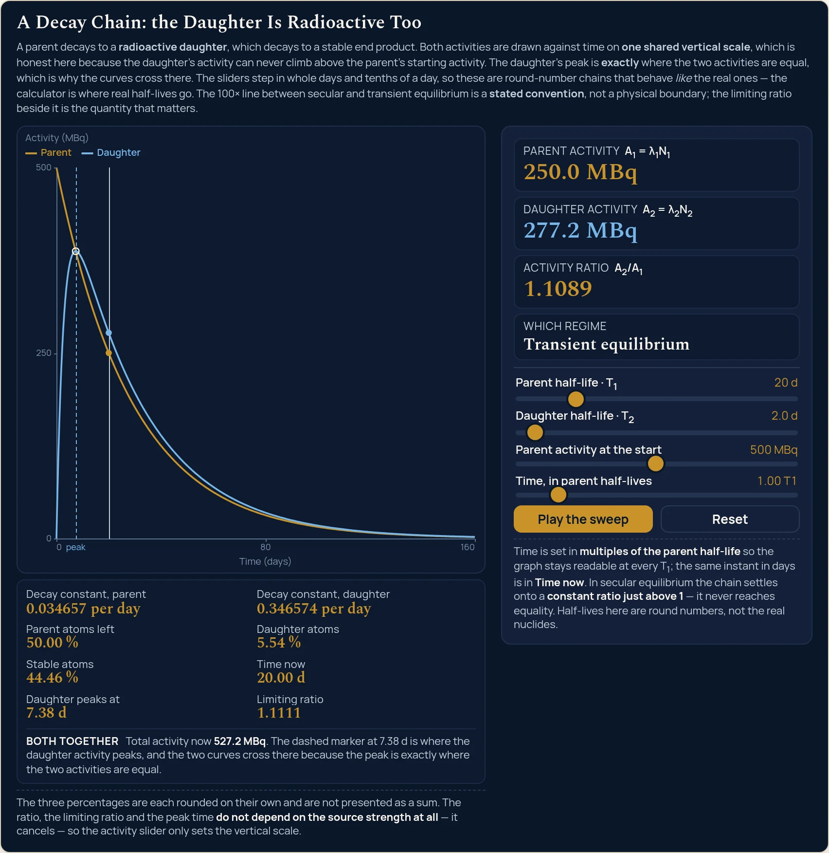
A parent decays to a radioactive daughter, which decays to a stable end product. Both activities are drawn against time on one shared vertical scale, which is honest here because the daughter's activity can never climb above the parent's starting activity. The daughter's peak is exactly where the two activities are equal, which is why the curves cross there. The sliders step in whole days and tenths of a day, so these are round-number chains that behave like the real ones — the calculator is where real half-lives go. The 100× line between secular and transient equilibrium is a stated convention, not a physical boundary; the limiting ratio beside it is the quantity that matters.
Decay constant, parent0.034657 per day
Decay constant, daughter0.346574 per day
Parent atoms left50.00 %
Daughter atoms5.54 %
Stable atoms44.46 %
Time now20.00 d
Daughter peaks at7.38 d
Limiting ratio1.1111
Both togetherTotal activity now 527.2 MBq. The dashed marker at 7.38 d is where the daughter activity peaks, and the two curves cross there because the peak is exactly where the two activities are equal.
The three percentages are each rounded on their own and are not presented as a sum. The ratio, the limiting ratio and the peak time do not depend on the source strength at all — it cancels — so the activity slider only sets the vertical scale.
Parent activity A1 = λ1N1
250.0 MBq
Daughter activity A2 = λ2N2
277.2 MBq
Activity ratio A2/A1
1.1089
Which regime
Transient equilibrium
Parent half-life · T120 d
Daughter half-life · T22.0 d
Parent activity at the start500 MBq
Time, in parent half-lives1.00 T1
Time is set in multiples of the parent half-life so the graph stays readable at every T1; the same instant in days is in Time now. In secular equilibrium the chain settles onto a constant ratio just above 1 — it never reaches equality. Half-lives here are round numbers, not the real nuclides.
Load a real chain on the sliders
Each button presses the lab's own Reset and then writes all four sliders, so every load starts from the same place and a running sweep is stopped before the new values land. Work down the list and watch the Which regime card change its mind three times. The last two names end in -like for a reason: the sliders move in whole days and tenths of a day, so they can stand in for a real chain without ever being one.
Pick a chain above, or drag the four sliders yourself.
What Is the Decay Chain Simulator?
The decay chain simulator is a free interactive physics lab that runs in your browser, with nothing to install and no sign-up. A parent nuclide decays to a radioactive daughter, and that daughter decays to a stable end product. Both activities are drawn against time on one shared vertical scale, and four sliders set the parent half-life from 1 to 100 d, the daughter half-life from 0.1 to 50.0 d, the parent activity at the start from 10 to 1000 MBq, and the clock from 0 to 8 parent half-lives.
The panel answers with the parent activity, the daughter activity, the activity ratio A2/A1 to four decimal places and which of three regimes the chain is in. Eight more cells carry both decay constants, the three atom percentages, the time in days, the time the daughter activity peaks and the limiting ratio the pair is heading for, with the total activity in a strip under the graph. Play the sweep runs the clock forward; Reset restores 20 d, 2.0 d, 500 MBq and 1.00 parent half-lives.
| Control | Range | Step |
|---|---|---|
| Parent half-life | 1 to 100 d | 1 d |
| Daughter half-life | 0.1 to 50.0 d | 0.1 d |
| Parent activity | 10 to 1000 MBq | 10 MBq |
| Time in parent half-lives | 0 to 8 | 0.02 |
| Play the sweep | runs the clock | one button |
| Reset | back to the start | one button |
How to use the radioactive decay chain simulator
- Start from the state it opens in. The lab boots at rest on 20 d, 2.0 d, 500 MBq and 1.00 T1, so every reading is already on the screen before you touch anything. Reset returns all four sliders to exactly that and stops the sweep if it is running.
- Set the parent half-life. Parent half-life · T1 runs from 1 to 100 d in whole days, and it stretches the horizontal axis with it, because the plot always covers eight of them. At 20 d the axis ticks read 0, 80 and 160; at 100 d they read 0, 400 and 800. If you want the single-nuclide version of that idea first, the guide to half-life and the decay constant covers it.
- Set the daughter half-life. Daughter half-life · T2 runs from 0.1 to 50.0 d in tenths. These two sliders together decide every shape on the screen; nothing else does. Put the daughter below the parent and it climbs and then follows; put it above and it never catches up.
- Choose how strong the source is. Parent activity at the start runs from 10 to 1000 MBq in steps of 10 and means the activity at the moment the daughter was last stripped out. It multiplies the two activity cards and the total in the strip, and it leaves the ratio, the ceiling, the peak time and the three percentages exactly where they were.
- Move the clock. Time, in parent half-lives runs from 0 to 8 in steps of 0.02, and the figure beside it reads in multiples of T1 rather than days. Time now gives you the same instant in days, so 1.00 T1 is 20.00 d on the opening chain and 13.00 d on the Ba-140-like one.
- Read the four cards down the right. Parent activity and Daughter activity carry their own formula lines,
A1 = λ1N1andA2 = λ2N2, in MBq to one decimal place. Activity ratio · A2/A1 carries four decimal places at every size it can reach, and Which regime carries one of exactly three phrases. - Read the eight cells under the graph. Both decay constants to six decimal places per day, the three atom percentages to two, then Time now, Daughter peaks at and Limiting ratio. That last one prints the word
nonerather than a number whenever the daughter is the longer-lived of the pair. - Read the strip below them. Total activity now is what a detector that cannot separate the two lines would see, and beside it a sentence names the peak. If the dashed marker is drawn the sentence points at it; if the peak sits too close to the vertical axis to mark, the sentence gives the time in words instead and says that no marker was drawn.
- Press Play the sweep to let the clock run. It advances four tenths of a parent half-life every second, wraps back to the start past the right-hand edge, and becomes Pause the sweep while it is going. Only the clock moves: the half-lives and the source strength stay where you put them.
When the daughter is stable, or its fate is not the thing you are after, this is more lab than you need. The half-life lab draws the single falling curve with nothing feeding it, which is the picture this one is built to contrast with. Come back here the moment the second nuclide starts to matter.
Worked example: change one thing at a time
Every row below is one setting of the four sliders, and every cell is a string the running lab printed there. The first two rows are the state it opens in and the nearest stop to its peak; the next four are the three regimes with a fourth chain that has no ceiling at all; the last four go looking for the corners. Where a cell and the lab ever part company, believe the lab.
| Setting | Sliders, as the panel reads them | Time now | Parent activity | Daughter activity | Activity ratio | Limiting ratio | Which regime | Daughter peaks at | Total activity |
|---|---|---|---|---|---|---|---|---|---|
| Opening state | 20 d · 2.0 d · 500 MBq · 1.00 T1 | 20.00 d | 250.0 MBq | 277.2 MBq | 1.1089 | 1.1111 | Transient equilibrium | 7.38 d | 527.2 MBq |
| Nearest stop to the peak | 20 d · 2.0 d · 500 MBq · 0.36 T1 | 7.20 d | 389.6 MBq | 387.1 MBq | 0.9935 | 1.1111 | Transient equilibrium | 7.38 d | 776.6 MBq |
| Secular, on the 100x line | 10 d · 0.1 d · 500 MBq · 1.00 T1 | 10.00 d | 250.0 MBq | 252.5 MBq | 1.0101 | 1.0101 | Secular equilibrium | 0.67 d | 502.5 MBq |
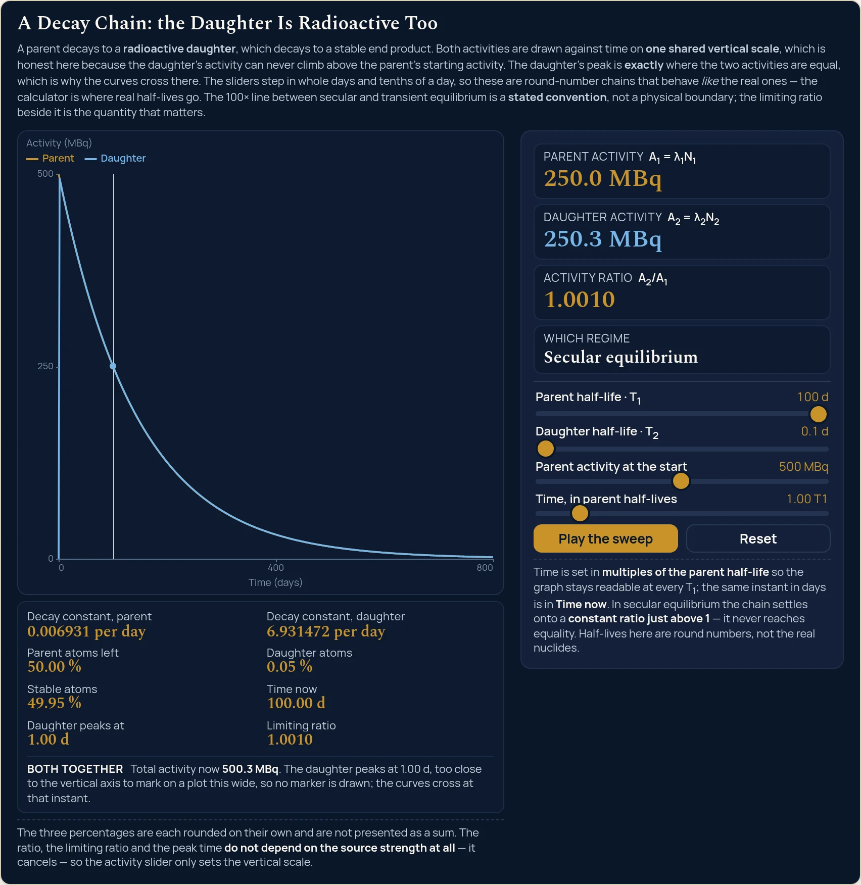
| Secular, deepest reachable | 100 d · 0.1 d · 500 MBq · 1.00 T1 | 100.00 d | 250.0 MBq | 250.3 MBq | 1.0010 | 1.0010 | Secular equilibrium | 1.00 d | 500.3 MBq |
| A Ba-140-like chain | 13 d · 1.7 d · 500 MBq · 1.00 T1 | 13.00 d | 250.0 MBq | 284.7 MBq | 1.1390 | 1.1504 | Transient equilibrium | 5.74 d | 534.7 MBq |
| A Bi-210-like inversion | 5 d · 50.0 d · 500 MBq · 1.00 T1 | 5.00 d | 250.0 MBq | 24.1 MBq | 0.0962 | none | No equilibrium | 18.46 d | 274.1 MBq |
| Equal half-lives | 20 d · 20.0 d · 500 MBq · 1.00 T1 | 20.00 d | 250.0 MBq | 173.3 MBq | 0.6931 | none | No equilibrium | 28.85 d | 423.3 MBq |
| The clock at zero | 20 d · 2.0 d · 500 MBq · 0.00 T1 | 0.00 d | 500.0 MBq | 0.0 MBq | 0.0000 | 1.1111 | Transient equilibrium | 7.38 d | 500.0 MBq |
| The far right edge | 20 d · 2.0 d · 500 MBq · 8.00 T1 | 160.00 d | 2.0 MBq | 2.2 MBq | 1.1111 | 1.1111 | Transient equilibrium | 7.38 d | 4.1 MBq |
| The smallest source | 20 d · 2.0 d · 10 MBq · 1.00 T1 | 20.00 d | 5.0 MBq | 5.5 MBq | 1.1089 | 1.1111 | Transient equilibrium | 7.38 d | 10.5 MBq |
| The largest source | 20 d · 2.0 d · 1000 MBq · 1.00 T1 | 20.00 d | 500.0 MBq | 554.5 MBq | 1.1089 | 1.1111 | Transient equilibrium | 7.38 d | 1054.5 MBq |
The two ratio columns are the pair to read together. One is where the chain stands now and the other is where it is going, and they are never the same question. On the Ba-140-like row the live ratio is 1.1390 while the ceiling is 1.1504; push that same chain on to 2.70 T1 and the live figure has crept up to 1.1504 as well, which is the ratio arriving rather than the two quantities being one thing.
Row 6 is the one with no ceiling. A parent of 5 d feeding a daughter of 50.0 d never settles into anything, so the Limiting ratio cell prints none instead of a number, and the daughter does not even reach its own peak until 18.46 d — by which time the parent, on a 5 d half-life, has very little left to give.
Row 7 is the case most textbook formulae cannot print. Give the parent and the daughter the same half-life and the usual expression divides by zero; this lab reads 0.6931 instead, because when the two decay constants match the ratio is simply the decay constant times the elapsed time. One parent half-life in, that product is ln 2.
Rows 1, 10 and 11 are the same chain at 10, 500 and 1000 MBq. The ratio, the ceiling, the peak time and the three percentages print identical strings in all three, and that agreement is not a result worth having: the source strength cancels out of every one of those quantities algebraically. What it tells you is narrower and more useful — the shape of a chain is set by the two half-lives, and the source only sets the height of the picture.
Rows 8 and 9 are the two ends of the clock. At 0.00 T1 the daughter has not been made yet, so its card reads 0.0 MBq and the ratio reads 0.0000. At 8.00 T1 the pair is down to 2.0 and 2.2 MBq and the live ratio prints 1.1111, the same four characters as the ceiling. If you need those figures for a real pair of half-lives rather than round ones, the decay chain calculator takes them to more decimal places and will run the sum backwards to date the sample.
Formula and symbol reference
The lab works from one relation. The ratio of the two activities is A2/A1 = λ2 t f((λ2 - λ1)t), where f(x) = (1 - e-x)/x and f(0) = 1. Written that way the difference of the two decay constants never sits underneath anything, which is why row 7 of the table above has an answer instead of an error.
Each decay constant is ln 2 divided by that member's half-life, so the two sliders you move and the two constants the panel prints carry the same information twice over. What kind of decay each step is never enters the arithmetic: a beta emitter and an alpha emitter with the same half-life draw the same pair of curves. The account of beta decay covers what is actually leaving the nucleus, which is the part this lab does not draw.
| Symbol | Meaning | SI unit | In this lab |
|---|---|---|---|
| T1 | Parent half-life. The time for half the parent atoms to go, and the unit the horizontal axis is counted in | second, s; the lab works in days | 1 to 100 in whole days, reading back as “20 d” after Reset. It sets the whole width of the graph: the plot always covers eight of these, so the axis ticks run to “160” at 20 d and to “800” at 100 d. |
| T2 | Daughter half-life. With the parent half-life it fixes every shape on the screen, and nothing else does | second, s; the lab works in days | 0.1 to 50.0 in tenths of a day; “2.0 d” after Reset. Taken alone to 0.1 d the regime card turns to Secular equilibrium and the ceiling reads “1.0050”; taken to 50.0 d it reads No equilibrium and the ceiling reads “none”. |
| A0 | Parent activity at the start. The strength of the source when the daughter was last stripped out | becquerel, Bq; the lab works in megabecquerels | 10 to 1000 in steps of 10; “500 MBq” after Reset. It scales the two activity cards and the total and nothing else: at 10 MBq the opening chain reads “5.0 MBq” and “5.5 MBq”, at 1000 MBq “500.0 MBq” and “554.5 MBq”, and the ratio is “1.1089” either way. |
| t/T1 | The clock, counted in parent half-lives so the picture stays the same shape whatever the half-life is | none — it is a ratio | 0 to 8 in steps of 0.02; “1.00 T1” after Reset. One step off zero is already visible: at “0.02 T1” the opening chain reads “493.1 MBq” and “64.3 MBq”. |
| t | The same instant in days. Printed as Time now, so you never have to do the multiplication yourself | second, s; the lab works in days | Two decimal places, from “0.00 d” to “160.00 d” on the opening chain. The same 1.00 T1 is “20.00 d” there and “13.00 d” on the Ba-140-like chain. |
| λ1 | Decay constant of the parent, which is ln 2 divided by its half-life. The chance per unit time that any one parent atom goes | per second; the lab prints per day | Six decimal places: “0.034657 per day” after Reset. The slider ends give “0.693147 per day” at 1 d and “0.006931 per day” at 100 d. |
| λ2 | Decay constant of the daughter, from its own half-life in the same way | per second; the lab prints per day | Six decimal places: “0.346574 per day” after Reset. The slider ends give “6.931472 per day” at 0.1 d and “0.013863 per day” at 50.0 d. |
| A1 | Parent activity now. The card carries its own formula line, A1 = lambda1 N1 | becquerel, Bq; the lab prints megabecquerels | One decimal place: “250.0 MBq” after Reset, “500.0 MBq” with the clock at zero and “2.0 MBq” at the far right edge. |
| A2 | Daughter activity now, from its own formula line A2 = lambda2 N2. It starts at nothing and has to be built | becquerel, Bq; the lab prints megabecquerels | One decimal place: “277.2 MBq” after Reset, “0.0 MBq” at the clock’s zero, and “554.5 MBq” at the top of the activity slider. |
| A2/A1 | Activity ratio. The one reading that says nothing about how strong your source is and everything about which chain it is | none — it is a ratio | Four decimal places everywhere it can go, with no magnitude switch at any size: “0.0000” at the clock’s zero, “1.1089” after Reset, and “21.0607” at 9 d against 38.9 d with the clock hard right. |
| rinf | Limiting ratio: the value A2/A1 is heading for, printed beside the regime name because it is the quantity that actually matters | none — it is a ratio | Four decimal places, or the word “none” when the daughter is the longer-lived of the two and there is nothing to head for. “1.1111” after Reset; “1.1504” on the Ba-140-like chain; “none” on the Bi-210-like one. |
| tmax | When the daughter activity peaks, which is the instant the two curves cross. Printed as Daughter peaks at | second, s; the lab prints days | Two decimal places: “7.38 d” after Reset, “5.74 d” on the Ba-140-like chain, “18.46 d” on the Bi-210-like one and “28.85 d” when the two half-lives match. |
| N1, N2, N3 | The three atom counts as percentages of the parent atoms you started with: parent left, daughter present, stable made | none — each is a percentage | Two decimal places each, rounded separately: “50.00 %”, “5.54 %” and “44.46 %” after Reset. At 13 d and 1.7 d with the clock on 1.30 T1 they read “40.61 %”, “6.09 %” and “53.29 %”. |
| A1 + A2 | Total activity now, in the strip under the graph. What a detector that cannot tell the two apart would be looking at | becquerel, Bq; the lab prints megabecquerels | One decimal place: “527.2 MBq” after Reset, “4.1 MBq” at the far right edge and “1054.5 MBq” at the top of the activity slider. |
Two of those rows deserve a second look. The Activity ratio card keeps four decimal places from 0.0000 right up to 21.0607, the largest figure these sliders can produce, with no switch to fewer digits at any size along the way. And none in the Limiting ratio cell is a real answer, not a gap: it is the lab declining to name a destination for a ratio that has none.
The physics: why the two curves cross at the daughter's peak
The daughter is being made and destroyed at the same moment. Its population changes at the parent's activity minus its own, so it grows for exactly as long as the parent is the stronger of the two and shrinks once it has overtaken. The turning point is therefore the instant the two activities are equal, which on a graph is the instant the two curves cross.
That is why the marker and the crossing are always at the same place, and why the caption under the graph says so in one sentence rather than two. On the opening state it reads: The dashed marker at 7.38 d is where the daughter activity peaks, and the two curves cross there because the peak is exactly where the two activities are equal.
You cannot quite land on it with the sliders, and that is worth knowing before you go hunting. The clock moves in steps of 0.02 T1, so on the opening chain the nearest stop to a peak at 7.38 d is 0.36 T1, which is 7.20 d. There the two cards read 389.6 MBq and 387.1 MBq and the ratio reads 0.9935 — near, and not the same.
After the peak the daughter stops keeping its own time. It is fed by a parent that is itself falling, so the pair lock into a fixed ratio and from then on both decline at the parent's rate. That fixed value is what the Limiting ratio cell has been printing all along, and the live ratio spends the rest of the graph creeping up to it.
How close that fixed value sits to 1 is the only thing separating the three names on the regime card. A parent far longer-lived than its daughter gives a ceiling barely above 1; a parent that still outlives its daughter but not by much gives one noticeably above 1; a parent that goes first gives no ceiling at all. The full account of decay chains works all three through with real nuclides and worked problems.
The hundredfold line between the first two names is a stated convention and nothing more. Nothing happens to the physics as a chain crosses it. The table below holds the daughter at 0.1 d and walks the parent across it one day at a time.
| Parent half-life | Daughter half-life | Which regime | Limiting ratio | Daughter peaks at |
|---|---|---|---|---|
| 9 d | 0.1 d | Transient equilibrium | 1.0112 | 0.66 d |
| 10 d | 0.1 d | Secular equilibrium | 1.0101 | 0.67 d |
| 11 d | 0.1 d | Secular equilibrium | 1.0092 | 0.68 d |
| 100 d | 0.1 d | Secular equilibrium | 1.0010 | 1.00 d |
| 20 d | 2.0 d | Transient equilibrium | 1.1111 | 7.38 d |
| 5 d | 5.0 d | No equilibrium | none | 7.21 d |
| 5 d | 50.0 d | No equilibrium | none | 18.46 d |
Nine days against a tenth of a day is called transient and eleven days is called secular, while the ceiling moves from 1.0112 to 1.0092 — about two parts in a thousand. The name changed; nothing measurable did. That is exactly why the lab prints the ceiling next to the name instead of leaving you with the word.
And the two activities never do become equal. Take the parent to 100 d against the same 0.1 d daughter, the deepest secular state these sliders reach, and both the Activity ratio and the Limiting ratio read 1.0010. They agree with each other to every digit printed, and neither of them is 1.0000. That last thousandth is not a rounding artefact: it is the margin by which the parent stays ahead, and the daughter is supplied out of it.
Where the decay chain model breaks down
The lab solves its own model exactly, so nothing on the screen ever fails. Everything below is a limit of that model, of the situation it stands for, or of the way the figures are printed, and each item says what the lab does about it.
- The daughter has to start at nothing
- Every curve here begins with the daughter absent, which is what the phrase since separation means. If your sample already held some of the daughter when your clock started, the true curve sits above this one by the amount that was there, decaying on its own schedule. There is no control for it, because the model has no term for it.
- Exactly three members, and no branches
- A parent, one radioactive daughter, one stable end. A nuclide that decays two ways at once splits into two partial paths, and this lab has no way to divide the flow between them. Bismuth-210, which one of the presets is named after, has a tiny alpha branch alongside its main beta route, and nothing on this page models it.
- Real series are much longer than three
- Uranium-238 runs a long way down to lead-206, and a natural series like that is a queue of chains rather than one. Each neighbouring pair in it behaves much as this lab shows, but the whole series does not, and a three-member tool cannot tell you what the eleventh member is doing. Look the intermediate half-lives up in published nuclear data rather than guessing them.
- The sliders cannot reach a published half-life
- The parent moves in whole days and the daughter in tenths, so barium-140 at 12.751 d and lanthanum-140 at 1.67858 d simply are not on the grid; 13 d and 1.7 d are the nearest stops, and that is why the preset says Ba-140-like. Bismuth-210 at 5.012 d misses a whole-day stop in the same way, which is why the inversion preset is Bi-210-like and never the nuclide itself. When the figures have to be the published ones, the decay chain calculator takes them exactly, in whichever time unit they were quoted in.
- Nothing here is counted, so nothing here is noisy
- These curves are smooth because the model is deterministic. A real measurement of the same chain is a count, and a count carries its own scatter that grows relatively worse as the activity falls. The far right of this graph, where the pair are down to a couple of megabecquerels, is exactly where a real detector would be struggling most and this drawing is at its most confident.
- The three percentages are rounded one at a time
- Parent atoms left, Daughter atoms and Stable atoms each get two decimal places of their own, so the printed trio need not close on 100.00. At 13 d and 1.7 d with the clock on 1.30 T1 they read 40.61, 6.09 and 53.29 per cent. The lab's own fixed note says they are not presented as a sum, and this page does not present them as one either.
- Recomputing one reading from another will usually not come out
- Activities are rounded to one decimal place and the ratio to four, each on its own, so dividing the two figures you can see rarely reproduces the ratio card exactly. On the opening state 277.2 divided by 250.0 gives 1.1088 against a printed 1.1089. The lab carries full precision internally and only the display is rounded.
- The far right of the graph is where the ratio stops moving
- Once the live ratio has crept up to the limiting ratio, later instants print the same four characters as each other. The far right of the opening chain reads 1.1089 at one parent half-life and 1.1111 at eight, and beyond that it has nowhere left to move. A measured ratio can date a sample only while it is still climbing.
- Every number here is a setting, not a measurement
- The four sliders are things you chose, and nothing in this lab has measured a source, a shipment or a sample. It will happily draw a 1000 MBq parent with a one-day half-life; whether such a thing sits in anybody's laboratory is a separate question the arithmetic has no view on.
Where decay chain readings are actually used
- Generators that supply a short-lived daughter
- A long-lived parent is held on a column and the daughter that grows in on it is washed off when it is wanted, after which it starts growing back. The shape of that regrowth is the daughter curve on this graph read from the left-hand edge, and the useful question is how long to wait before the next draw. Load Secular, deepest reachable to see the limiting case, where the daughter comes back almost to the parent's own activity.
- Radon indoors is a daughter, not a source
- Radon-222 has a half-life of 3.8235 d, which is far too short for any of it to be left over from the formation of the rock. It is there because radium-226, at 1600 y, is in the ground making more of it, which is the same parent-feeding-daughter arrangement this lab draws. That is also why airing a room out once does not settle it: the supply in the ground has not been touched, so the gas builds back up along the same climb this lab draws from the left-hand edge of the graph.
- Dating a sample from the ratio of two lines
- If you can measure the parent and the daughter separately, the ratio between them is a clock, because on a chain that has not yet reached its ceiling each elapsed time gives a different value. That is a different method from counting how much of one nuclide is left, which is what radiocarbon dating does, and it needs no assumption about the starting amount.
- A fission-product pair that arrives still growing
- A barium-140 and lanthanum-140 pair is a fission product that arrives at a laboratory still building its daughter, so the dose rate from a freshly separated batch goes up before it goes down. Load A Ba-140-like chain and run the sweep to watch that happen. The reactor lab shows where such pairs come from in the first place.
- Shielding a source that is really two sources
- The Total activity now figure in the strip is what an instrument that cannot separate the two nuclides responds to, and on the opening state it is 527.2 MBq against a parent of 250.0 MBq. Planning around the parent alone understates it by more than a factor of two. The two nuclides also rarely emit at the same energy, so the shielding calculation is genuinely two calculations.
- Checking a delivered source against its quoted date
- A delivered source is quoted at an activity on a date, and if its daughter was separated at that moment the pair have been growing together ever since. Setting the two half-lives and the elapsed time here gives the shape of what should have happened; the half-life calculator is the right tool instead when the daughter is stable and one curve is the whole story.
- Teaching which curve is which
- Chain problems go wrong when a student reads the daughter curve as though it were a second parent curve. Drag the daughter half-life from 0.1 d up to 50.0 d and watch the same picture turn from two lines lying on top of one another into a late, low hump that peaks long after the parent has gone. That is hard to see on paper and immediate here.
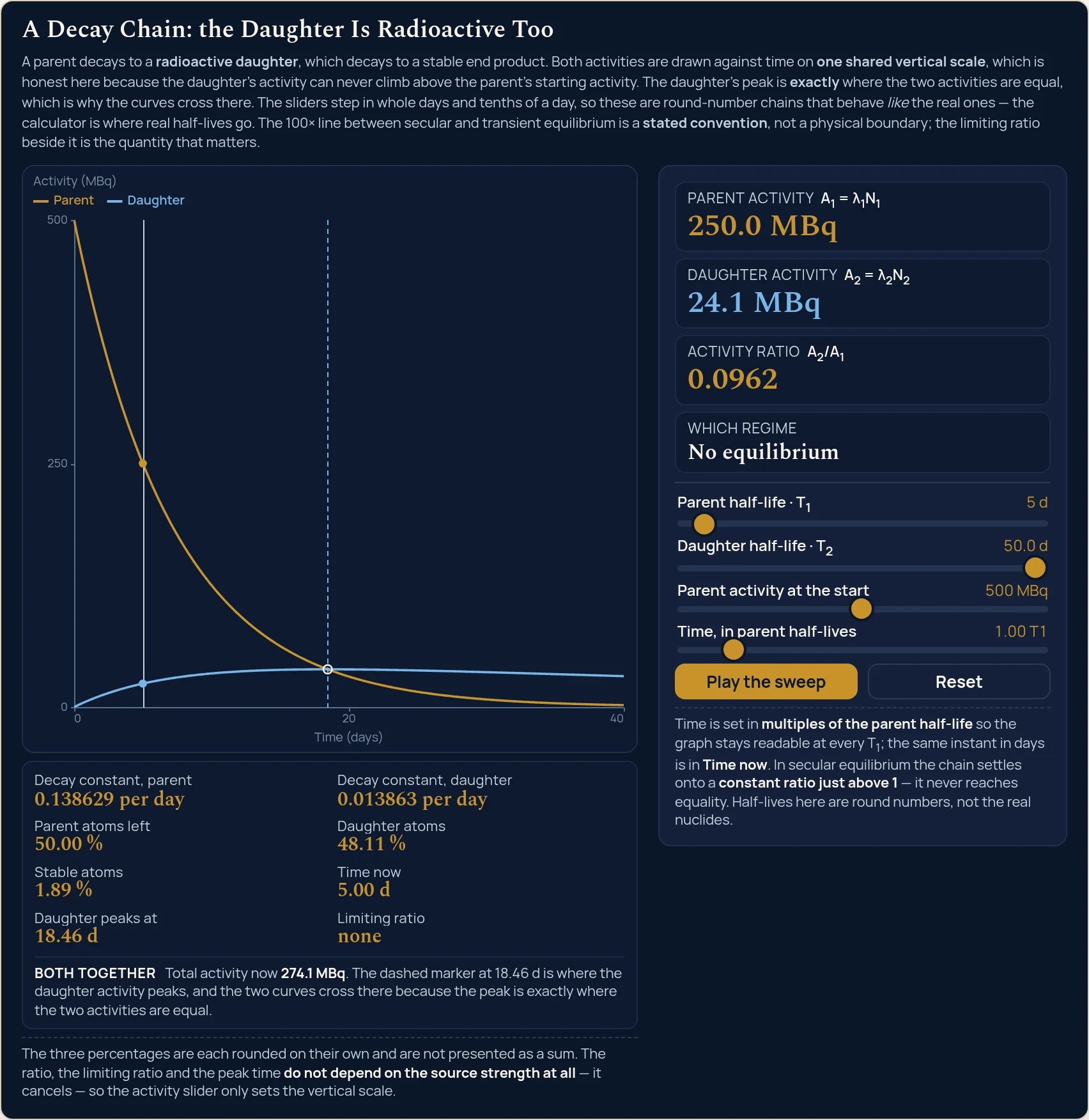
none — there is nothing for the ratio to settle onto. The daughter does not peak until 18.46 d, by which time the parent curve has flattened onto the floor of the graph.Where to go next
For the method itself, with the three regimes worked through on real nuclides, eight problems of rising difficulty and the diagrams that go with them, read Radioactive Decay Chains Explained. If you would rather type published half-lives than drag sliders, or you need the sum run backwards to date a sample, the calculator is the first card under Related tools below.
The single-nuclide background this lab assumes is in What Is Half-Life in Physics?, with the half-life lab and the half-life calculator beside it. For what is actually being emitted at each step there is Beta Decay Explained, Gamma Rays: Properties and Uses and the survey in Radioactivity: Alpha, Beta and Gamma.
Further afield, Carbon Dating: The Physics Behind It and the carbon dating lab take the dating idea the other way about, while How a Nuclear Reactor Works and Fission vs Fusion cover where fresh chains come from. The rest of the collection is in the library of physics simulations and on the blog, and the site search will find a topic by name.
Frequently asked questions
Why does the daughter line start at nothing?
Because the lab starts you the moment the daughter was last stripped out. That is what the model assumes, and it is why the daughter has to be made before it can decay: at a clock reading of 0.00 T1 the daughter activity card reads 0.0 MBq and the ratio reads 0.0000. Drag the clock a single step, to 0.02 T1, and the same card already reads 64.3 MBq.
Why is the clock in parent half-lives rather than days?
So the picture stays readable whatever half-life you choose. The graph always spans eight parent half-lives, so a chain of 1 d and a chain of 100 d both fill the width instead of one of them collapsing onto the axis. The day figure is never hidden from you: Time now prints the same instant in days, so 1.00 T1 reads 20.00 d on the opening state and 13.00 d on the Ba-140-like one.
In secular equilibrium, do the two activities end up equal?
No, and this lab is built so you can see that they do not. Take the sliders to the deepest secular state they reach, a parent of 100 d against a daughter of 0.1 d: the Activity ratio card reads 1.0010 and the Limiting ratio beside it reads 1.0010. Those are the same string as each other and neither of them is 1.0000. The gap is what keeps the daughter supplied.
Why does the dashed peak marker sometimes vanish?
Because it would be drawn on top of the vertical axis, where it would read as part of the axis rather than as a measurement. The lab tests the position in pixels on the plot it is actually drawing and drops the marker when it falls within three pixels of the axis. Nothing is lost: the caption under the graph then gives the peak time in words instead, to the same two decimal places.
Should the three atom percentages add up to 100?
Not always, and the lab says so in its own fixed note. Parent atoms left, Daughter atoms and Stable atoms are each rounded to two decimal places on their own, so the printed figures need not close. At 13 d and 1.7 d with the clock at 1.30 T1 they read 40.61, 6.09 and 53.29 per cent, which comes to 99.99. Read them one at a time.
Why does the activity slider change so little?
Because it only sets the vertical scale. Parent activity at the start multiplies the two activity cards and the total in the strip, and the strength cancels out of everything else algebraically. Run the opening chain at 10 MBq and at 1000 MBq and the ratio, the limiting ratio, the peak time and the three percentages print the same strings both times, while the activities go from 5.0 and 5.5 MBq up to 500.0 and 554.5 MBq.
What is the biggest activity ratio these sliders can reach?
The four decimal places on the Activity ratio card go up to 21.0607, at a parent of 9 d, a daughter of 38.9 d and the clock at the far right of its travel. The card has no magnitude switch anywhere in that range, so the figure keeps four decimal places at 0.0000, at 1.1089 and at 21.0607 alike. The regime card reads No equilibrium there and the limiting ratio reads none.
What does none mean in the Limiting ratio box?
It means the ratio is not heading for anything, so there is no number to print. A ceiling exists only when the parent outlives the daughter. Set a parent of 5 d against a daughter of 50.0 d and the box reads none, because the daughter is the slower of the pair and the ratio climbs for as long as there is a parent left. Equal half-lives read none as well.
Can I put a real nuclide into these sliders?
Not exactly, and the preset names say so by calling their chains Ba-140-like and Bi-210-like rather than naming the nuclides outright. The parent slider steps in whole days and the daughter slider in tenths of a day, so a published half-life such as 12.751 d cannot be dialled in. Use the decay chain calculator when the figures have to be the real ones.
What does Play the sweep actually move?
Only the clock. It advances Time, in parent half-lives at four tenths of a parent half-life every second, redrawing the cursor and every reading as it goes, and it wraps back to the start once it passes the right-hand edge. The half-lives and the source strength stay exactly where you left them, and the button becomes Pause the sweep while it runs.
References & formula source
- Krane, Introductory Nuclear Physics: successive decays and the Bateman solution, for the three-member chain this lab draws and the conditions under which each equilibrium name applies.
- Knoll, Radiation Detection and Measurement: activity, counting statistics and why a deterministic curve is the mean of a process that a real detector only samples.
- Lilley, Nuclear Physics: Principles and Applications: the natural decay series and the difference between a chain that reaches equilibrium and one that never can.
- Every half-life named on this page is a published ground-state value from the IAEA Nuclear Data Services ground-state table, retrieved 2026-09-20: barium-140 12.751 d, lanthanum-140 1.67858 d, bismuth-210 5.012 d, radon-222 3.8235 d and radium-226 1600 y, with lead-206 stable. Uranium-238 is named as the head of the long natural series and no half-life is quoted for it or for any member between it and lead-206.
- Every figure on this page is a reading this simulation printed for a setting of its own sliders. The sliders step in whole days and tenths of a day, so no state of this lab is a real nuclide, and none of these numbers describes a particular source, sample or shipment. Verify against your own measurement and your own published data before use.
- Further reading: Decay chain — Wikipedia