Carbon dating reads a clock that starts at death: the carbon-14 in a living thing is topped up from the air, the topping-up stops when it dies, and what survives fixes the interval through t = (t½ / ln 2) · ln(N0 / N). The answer is a radiocarbon age in years before 1950, not a calendar date. This lab puts the three quantities that decide it under your hands — what a laboratory measured, what the atmosphere held when the organism died, and how precise the measurement was — and prints the age, its range, the carbon-14 remaining and the half-lives elapsed. Press one of the three half-life buttons and every age rescales while the measurement stays put.
Carbon Dating: Reading the Carbon-14 Clock
While an organism is alive it keeps its carbon-14 topped up by exchange with the atmosphere. When it dies the exchange stops and the carbon-14 decays, so the surviving fraction dates the death: age = (T / ln 2) · ln(N0 / N), where T is the half-life of carbon-14. Set what the laboratory measured, what the atmosphere held when the organism died, and how precise the measurement was. The panel reports the radiocarbon age — years before 1950, on the assumption that the atmosphere always held the 1950 level, which it did not. Turning that into a calendar date needs a published calibration curve, and this lab does not carry one.
Half-lives elapsed1.000 half-lives
Mean lifetime tau8,223 yearsmean lifetime: T divided by ln(2)
Decay constant0.00012160 per yeardecay constant: ln(2) divided by T
Practical limit of the methodabout 50,000 yearswhere the reading runs into laboratory background
The other two half-livesSame measurement on the other two half-lives: 5730 y: 5,730 · 5568 y: 5,570 radiocarbon years.
What the half-life means hereEach 5,700 years halves what is left: after 1.000 half-lives, 50.00 % of the starting carbon-14 is still there.
What the reading meansRadiocarbon years, not calendar years: the atmosphere has not always held exactly the 1950 level, so a published calibration curve is needed to turn this into a calendar date.
Fixed by the physics: age = -(T / ln 2) ln(f), with f the measured level divided by the atmospheric level when the organism died. Published half-lives: 5700 y (currently recommended) · 5730 y (Cambridge) · 5568 y (Libby, kept by convention so reported ages stay comparable). A radiocarbon age is not a calendar age.
Radiocarbon age age = -(T / ln 2) ln(f)
5,700 radiocarbon years BP
5,660 to 5,740 radiocarbon years BP
Uncertainty in the age
± 41 years
one standard deviation from the measurement alone
Carbon-14 remaining f = pMC / atmosphere
50.00 %
of the carbon-14 it started with
Half-life in use
5700 years
the currently recommended value
Measured carbon-1450.0 pMC
percent of the 1950 modern standard
Atmosphere when it died100 pMC
100 is the 1950 standard
Measurement uncertainty± 0.5 % of the reading
this moves the range, never the age
Half-life used
Load a sample
custom sample
Tip: load the ice-age bone, then drag the uncertainty from 1.0 % to 5.0 %. The age never moves — only the range does. Then press 5568 y: the age changes, but the measurement does not.
Load a real measurement
The first five presets press the lab's own sample buttons, which set all three sliders at once and name the case on the panel. The last three write the sliders directly, so the sample line stays at custom sample. Every caption is what the lab then prints on the 5700-year half-life, which is where Reset leaves it.
Pick a measurement above, or drag the sliders yourself.
What Is the Carbon Dating Simulator?
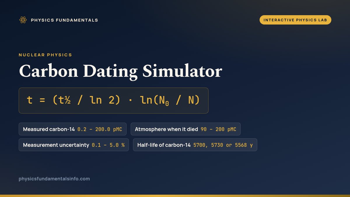
The carbon dating simulator is a free interactive physics lab that runs in your browser — nothing to install and no sign-up. Set the measured carbon-14 level anywhere from 0.2 to 200.0 pMC, say what the atmosphere held when the organism died, from 90 to 200 pMC, and choose a measurement uncertainty between 0.1 and 5.0 % of the reading. The panel answers with the radiocarbon age in years before 1950, the range around it, the fraction of carbon-14 still present and the number of half-lives elapsed, on whichever of the three half-lives you press.
| Control | Range | Step |
|---|---|---|
| Measured carbon-14 | 0.2 – 200.0 pMC | 0.1 |
| Atmosphere when it died | 90 – 200 pMC | 1 |
| Measurement uncertainty | 0.1 – 5.0 % | 0.1 |
| Half-life of carbon-14 | 5700, 5730 or 5568 y | buttons |
How to use the carbon dating simulator
- Load a sample. The five buttons under Load a sample — Freshly dead, One half-life, Old hearth charcoal, Ice-age bone and At the limit of the method — set all three sliders and name the case on the line below them, for instance Charcoal from an old hearth. Touch any slider and that line reverts to custom sample. Reset returns to 50.0 pMC, 100 pMC, ± 0.5 % and the 5700-year half-life.
- Set what the laboratory measured. Drag Measured carbon-14 anywhere from 0.2 to 200.0 pMC in steps of 0.1, and the figure beside it reads back as “25.0 pMC”. Radiocarbon age answers at once, and the gold ring labelled this sample moves to the point on the decay curve where that reading meets that age.
- Say what the atmosphere held. Atmosphere when it died runs from 90 to 200 pMC in whole units and is the denominator of everything: Carbon-14 remaining is the measured level divided by it. Move it off 100 and a dotted line labelled atmosphere when it died appears on the chart, and the note line tells you how far the age would shift if you assumed 100 instead — unless the reading is post-1950 or near the limit, which the note reports first.
- Set how good the measurement was. Measurement uncertainty covers 0.1 to 5.0 % of the reading. It drives Uncertainty in the age, the range printed under the age and the width of the gold band on the chart — and it never moves the age itself, which is the single most useful thing this lab proves.
- Declare a half-life. The three buttons under Half-life used — 5700 y, 5730 y and 5568 y — change Half-life in use, Mean lifetime, Decay constant, the age, its range and the slope of the line. They leave Carbon-14 remaining alone, because a half-life is a fixed property of the isotope rather than anything your sample decides — the constancy that half-life physics builds the decay law on. The other two half-lives spells out what the same reading would have given on the buttons you did not press.
- Read the lab's own commentary, printed under the chart. What the half-life means here puts the reading into halvings, What the reading means switches between five notes as the setting crosses each boundary, and Practical limit of the method never moves at all. Pause stops the decay animation without touching a single number.
Worked example: change one thing at a time
Start from the state the lab boots in — 50.0 pMC measured, a 100 pMC atmosphere, ± 0.5 % of the reading, 5700 years — and move one control per row. Every cell below is a string the running lab printed at those control positions; where a cell and the lab disagree, the lab is right. Only the last row presses a button rather than dragging a slider.
| Step | Sliders: measured, atmosphere, uncertainty | Half-life in use | Radiocarbon age | Uncertainty in the age | Carbon-14 remaining | Half-lives elapsed |
|---|---|---|---|---|---|---|
| Start: the state the lab boots in | 50.0 pMC · 100 pMC · ± 0.5 % | 5700 years | 5,700 radiocarbon years BP | ± 41 years | 50.00 % | 1.000 half-lives |
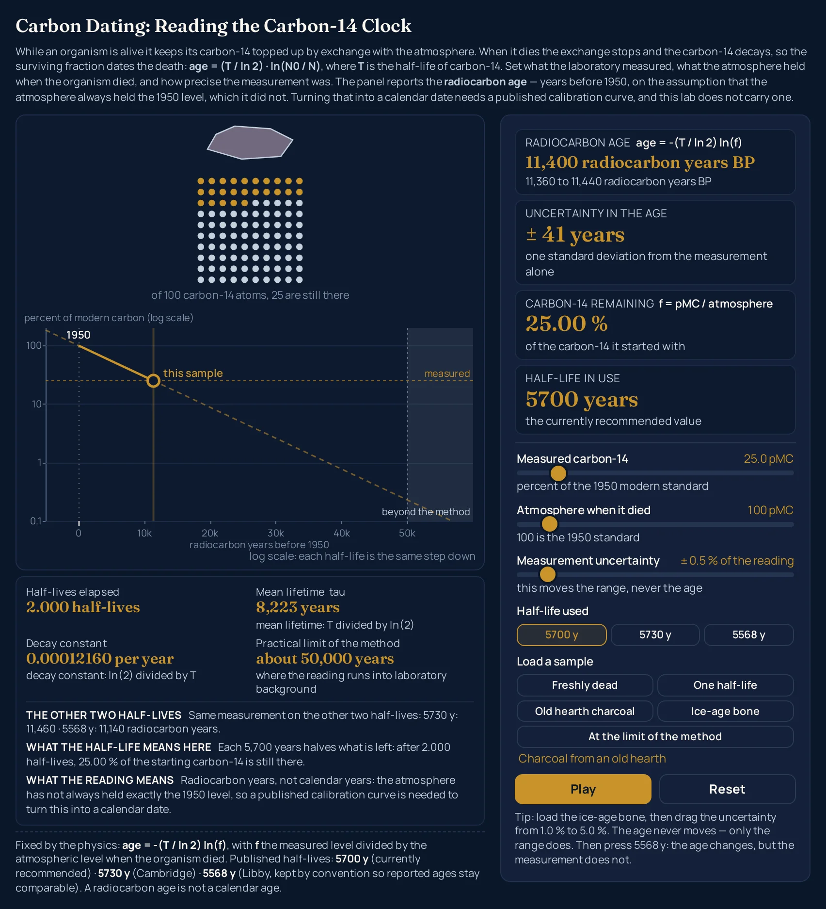
| Halve the reading to 25.0 pMC | 25.0 pMC · 100 pMC · ± 0.5 % | 5700 years | 11,400 radiocarbon years BP | ± 41 years | 25.00 % | 2.000 half-lives |
| Widen the uncertainty to 2.0 % | 25.0 pMC · 100 pMC · ± 2.0 % | 5700 years | 11,400 radiocarbon years BP | ± 164 years | 25.00 % | 2.000 half-lives |
| Press the 5568 y button | 25.0 pMC · 100 pMC · ± 2.0 % | 5568 years | 11,140 radiocarbon years BP | ± 161 years | 25.00 % | 2.000 half-lives |
Row 2 shows that the reading sets the age. Halving the measured level adds exactly one halving: the count goes from 1.000 to 2.000 half-lives and the age from 5,700 to 11,400 radiocarbon years BP. Nothing else was touched. That is the whole method in one drag, and it is the one case you can check in your head — or in the half-life calculator, which solves the same equation for whichever of its four quantities you leave out.
Row 3 shows that precision sets only the bar. Four times the uncertainty leaves the age at 11,400 radiocarbon years BP and takes the range from “11,360 to 11,440” out to “11,240 to 11,570 radiocarbon years BP”, with Uncertainty in the age going from ± 41 to ± 164 years. Notice that the range is lopsided: 160 years below the age and 170 above it, because a shortfall in carbon-14 costs more years than the same surplus saves.
Row 4 shows that the half-life is a declaration. Pressing 5568 y drops the age to 11,140 radiocarbon years BP and the mean lifetime from 8,223 to 8,033 years, while Carbon-14 remaining sits unmoved at 25.00 % and the count at 2.000 half-lives. The physics contract behind this lab puts the gap between the 5568 and 5730-year answers at 2.9095 % of the Libby age, at every reading. An age quoted without its half-life is ambiguous by that much.
A fixed relative precision is a fixed number of years. Leave the uncertainty at ± 0.5 % and walk the measured level from 50.0 pMC down to 0.2 pMC: Uncertainty in the age reads ± 41 years at both ends, and everywhere between. Old dates are less precise in practice because there is so little carbon-14 left that the percentage itself gets worse — which is the slider you have to move yourself.
Formula and symbol reference
The lab divides the measured level by the atmosphere to get the surviving fraction, takes its logarithm, multiplies by the mean lifetime and rounds to the nearest 10 years, which is the convention for a reported radiocarbon age. Ranges marked “in this lab” are the controls' own ends and the strings the lab prints there; to watch the same law run forwards on a half-life you set yourself, counting atoms rather than a percentage of a standard, use the half-life simulator.
| Symbol | Meaning | SI unit | In this lab |
|---|---|---|---|
| t | Radiocarbon age: the years before 1950 the decay law returns for this reading | second, s (printed in years) | From -6,600 radiocarbon years BP (200.0 pMC on a 90 pMC atmosphere, 5730 y) to 57,100 (0.2 pMC on a 200 pMC atmosphere, 5730 y). Always rounded to the nearest 10 years, and a value that rounds to zero prints “0 radiocarbon years BP”. |
| t½ | Half-life of carbon-14: the convention this answer is computed on, and which you must declare | second, s (shown in years) | Three buttons, no slider: 5700 years after Reset, 5730 years and 5568 years. The panel names each one — the currently recommended value, the Cambridge value used by our half-life calculator, and the Libby value kept by convention for reported ages. |
| N | Measured carbon-14: what the laboratory reports, as a percentage of the 1950 modern standard (pMC) | none (a ratio, shown as pMC) | 0.2 to 200.0 pMC in steps of 0.1; 50.0 pMC after Reset. This is the only control the age really needs, and it is the one that moves it. |
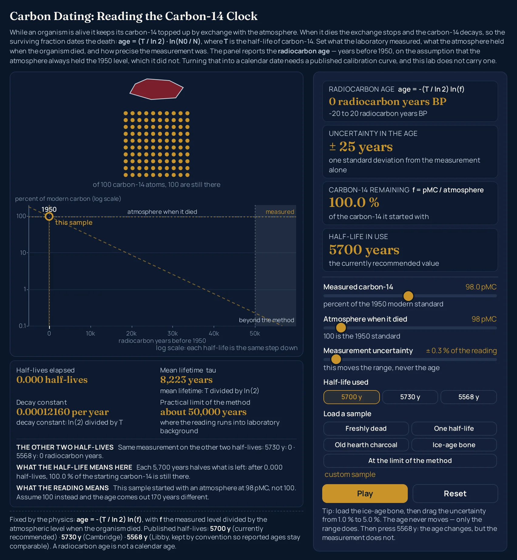
| N0 | Atmosphere when it died: the level the organism started from, on the same percentage scale | none (a ratio, shown as pMC) | 90 to 200 pMC in whole units; 100 pMC after Reset. It is the denominator, not decoration: 98.0 pMC read against 98 pMC gives 0 radiocarbon years BP, and read against 100 pMC gives 170. |
| f | Carbon-14 remaining: the measured level divided by that atmosphere | none (a ratio, shown as a percentage to four significant figures) | From 0.1000 % to 222.2 %. No half-life button changes it. Anything above 100 % means the sample holds more carbon-14 than its atmosphere did, and the age goes negative. |
| n | Half-lives elapsed | none (a count) | From -1.152 to 9.966 half-lives, always to three decimal places. Do not round it and then multiply: on the ice-age bone the lab prints 4.322 half-lives and 24,630 radiocarbon years BP, while 4.322 × 5700 would give 24,640. |
| τ | Mean lifetime, tau: the half-life divided by ln(2), and the constant that turns a percentage into years | second, s (shown in years) | 8,033 years, 8,223 years or 8,267 years, for the 5568, 5700 and 5730-year buttons. No slider moves it. |
| λ | Decay constant, lambda: ln(2) divided by the half-life | per second (shown per year) | 0.00012449, 0.00012160 or 0.00012097 per year, to five significant figures, again fixed by the button alone. |
| ± % | Measurement uncertainty: one standard deviation, as a percentage of the reading | none (a percentage) | 0.1 to 5.0 % in steps of 0.1; ± 0.5 % after Reset. On the 5700-year half-life it gives ± 8 years at one end and ± 412 years at the other, at every age. |
| Limit | Practical limit of the method: where the reading runs into laboratory background | second, s (shown in years) | Fixed at “about 50,000 years” at every setting of every control. The sliders go past it deliberately: 0.2 pMC on a 100 pMC atmosphere already reads 51,100 radiocarbon years BP. |
The physics: why a dead organism carries a clock
A living thing swaps carbon with its surroundings fast enough to hold whatever level the air holds, so its carbon-14 is continually restocked. Death ends the restocking, and from then on the only thing happening is decay: one carbon-14 nucleus at a time emits a beta-minus electron and an antineutrino and becomes nitrogen-14, which is the decay the beta decay simulator fires and counts. The lab starts at that moment: the Atmosphere when it died slider is the level it was holding when the swapping stopped, and Measured carbon-14 is what is left of it now.
Everything the lab prints follows from the ratio of those two numbers. Carbon-14 remaining is the division itself, Half-lives elapsed is how many times that fraction has halved, and the age is the halvings multiplied out. A percentage of a standard is all the method ever needs, which is why no count per minute, no gram of sample and no activity constant appears anywhere in this lab.
The chart puts carbon-14 on a logarithmic axis, with gridlines at 0.1, 1, 10 and 100, and that choice is what makes the exponential a straight line. One decade of that axis is always the same distance, so successive halvings land at a constant spacing instead of crowding together as the curve flattens. Drag the measured level and the gold ring slides along a line whose slope belongs to the half-life button, not to the sample.
Mean lifetime is the quiet constant behind the error bar. Because the uncertainty is a percentage of the reading, and a percentage becomes a fixed number of years once multiplied by the mean lifetime, ± 0.5 % is ± 41 years at 5,700 radiocarbon years BP and the same ± 41 years at 51,100. Press 5568 y and the mean lifetime falls to 8,033 years, so the same ± 0.5 % becomes ± 40 years instead.
Where carbon dating breaks down
The lab solves the decay law exactly, so on screen the method never fails. Every limit below is a limit of the real measurement, and each item says what the lab does about it.
- Nothing starts the clock except carbon going out of contact with the air
- What these sliders time is the interval since a parcel of carbon stopped exchanging carbon with the atmosphere. For an organism that moment is death, which is the overwhelmingly common case and the one this lab is built around; for deep water it is the moment that water sank away from the surface; for a rock it never happened at all, so there is nothing in it to read and no setting of these sliders changes that. The largest count the lab can reach is 9.966 half-lives; a dinosaur fossil is thousands of half-lives past death, with no carbon-14 left to measure at all, and is dated instead from the rocks around it.
- The ceiling is a measurement limit, not an equation
- Practical limit of the method reads about 50,000 years at every setting, with where the reading runs into laboratory background under it. The sliders deliberately go past it: at 0.2 pMC the panel still prints 51,100 radiocarbon years BP, and the note line changes to warn that a tiny error in the measurement, or a trace of modern carbon, moves the age by thousands of years. The number is a practical ceiling, and nothing in the equation puts a boundary anywhere.
- Contamination is brutal at the old end and harmless at the young one
- Drag the measured level from 1.0 to 2.0 pMC, which is what doubling a faint reading looks like, and the age falls from 37,870 to 32,170 radiocarbon years BP — a whole half-life younger. Do the equivalent at the fresh end, 50.0 pMC to 50.5 pMC, and the whole cost is 80 years: 5,620 radiocarbon years BP where the clean sample gave 5,700. The physics contract works the exact mixing case: 1 % of modern carbon in a 1.0 pMC sample reads 1.99 pMC and dates to 32,210 years, which is 5,660 years younger. That reading is off the 0.1 grid, so the lab cannot be set to it.
- A starting level of 100 is an assumption, not a fact
- This is the whole point of the second slider. Wood grown when the air held 98 pMC dates to 0 radiocarbon years BP on its own atmosphere, and to 170 radiocarbon years BP if you leave the slider at 100 — the lab's note line prints that difference for you. Burning fossil carbon diluted the air through the industrial period, and weapons testing later roughly doubled the carbon-14 in it, which is what puts the top of the slider at 200 pMC. The 90 pMC end carries no claim about the size of that dilution: it is headroom for starting an organism below the 1950 standard, which is what the reservoir item below asks you to do with it.
- Reservoir effects, which this lab has no control for
- Carbon that has been out of contact with the air for a long time makes an organism start below the atmospheric level: marine life and the animals that eat it, fresh water fed by old limestone, and settings near volcanic gas. Such a sample reads older than it is, and the honest way to mimic that here is to lower the Atmosphere when it died slider yourself. How far is a question this page cannot answer: the size of the offset varies with place and setting, and no figure for it was sourced for this lab.
- A radiocarbon age is not a calendar date
- The default note line says so outright: the atmosphere has not always held exactly the 1950 level, so a published calibration curve is needed to turn the answer into a calendar date. This lab carries no calibration curve, draws none, and converts nothing, and what the “BP” in its answers is counting back from is set out in why radiocarbon ages are quoted in years BP. What it gives you is the raw output of the decay law on a stated half-life, which is exactly what a laboratory reports before calibration — a reproducible number, and not yet a date.
- The lab's own arithmetic and display
- Ages are rounded to the nearest 10 years, so a rounded intermediate can mislead: 4.322 half-lives times 5700 comes to 24,640, while the panel prints 24,630 radiocarbon years BP. Carbon-14 remaining carries four significant figures and the half-life count three decimals. The measured slider steps by 0.1 pMC from 0.2, so four half-lives at 6.25 pMC is unreachable; 6.2 pMC gives 22,870 radiocarbon years BP and 6.3 pMC gives 22,730.
- What the drawing will not show you
- The chart spans -5,000 to 60,000 radiocarbon years, and a strongly post-1950 reading runs off the left-hand end of it. On the 5700-year half-life that happens as soon as the measured level passes about 1.84 times its atmosphere: 200.0 pMC against a 100 pMC atmosphere already gives -5,700 radiocarbon years BP, so the ring and its label are withheld rather than parked at the edge, while the panel keeps the number. The flashing dot in the grid is an animation of decay already counted, never a change to the tally, and Pause leaves the gold dots exactly as they were.
Where carbon dating is actually used
- Archaeology and museum conservation
- Charcoal, bone, seeds, textile and leather are the method's home ground, and the Old hearth charcoal button is that job in miniature: 25.0 pMC, 11,400 radiocarbon years BP, ± 41 years, on the 5700-year half-life the lab boots with — the half-life behind every age in this section that does not name another. A real report would name the half-life it used and pass the result through a calibration curve before anyone called it a date. Both of those steps are visible here as things the lab does not do for you.
- Recent remains, dated by the bomb rise
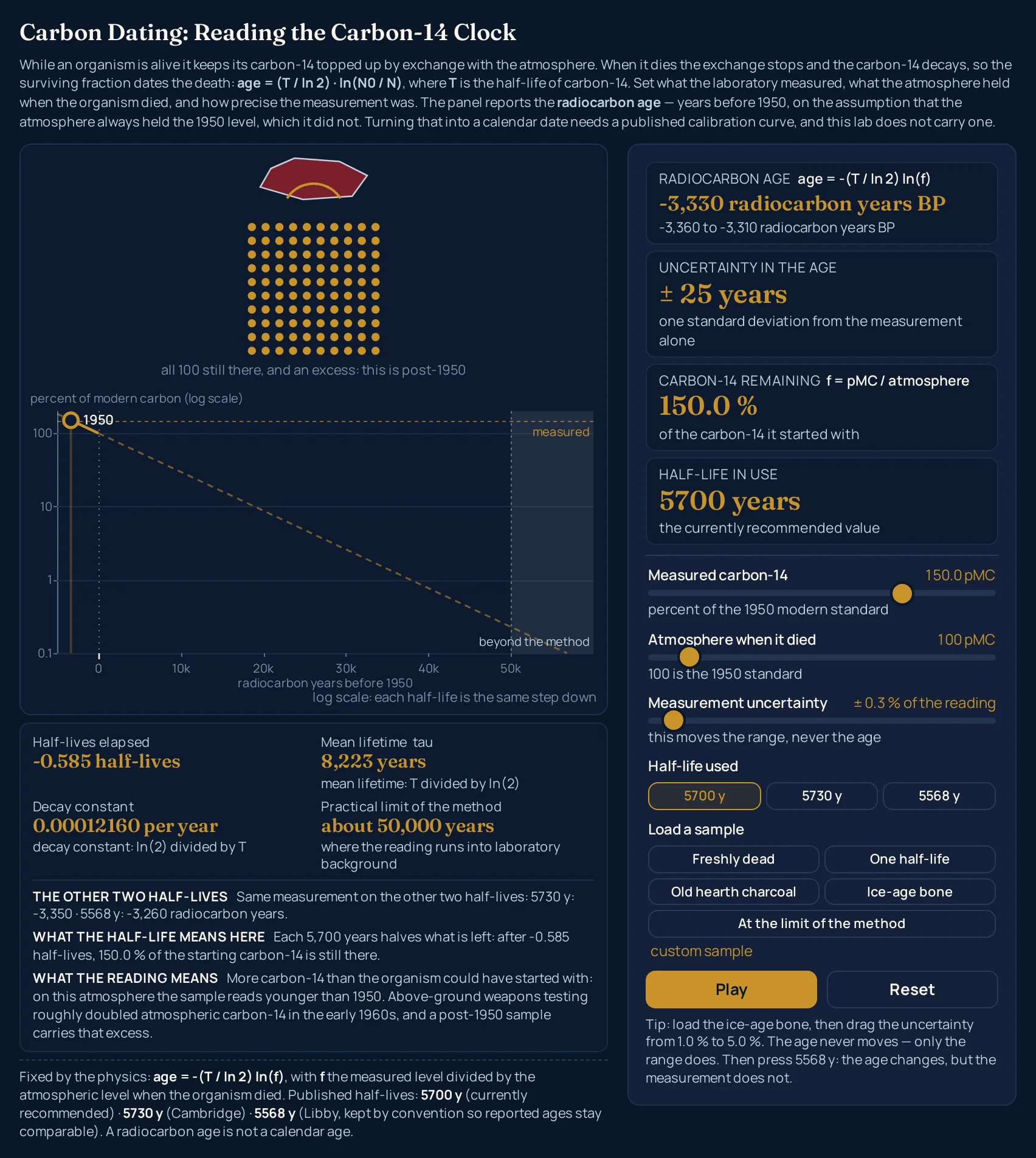
- Push the measured level above the atmosphere and the age goes negative: 150.0 pMC reads -3,330 radiocarbon years BP, with the note line explaining that above-ground weapons testing roughly doubled atmospheric carbon-14 in the early 1960s. That sharp rise and its slow fall since make the second half of the twentieth century unusually easy to place, which is what forensic work on recent material leans on. The lab gives you the arithmetic, not the calendar.
- Tracing water and ocean circulation
- Deep water is the other place where the exchange with the air stops cleanly, so the same stopwatch runs in it. Water that sank out of contact with the surface carries the level it had when it went down, and how far that level has decayed says how long it has been out of touch. The Atmosphere when it died slider is exactly the knob that idea needs: it lets you start the clock from something other than the 1950 standard.
- Checking whether organic material is genuinely old
- Press Freshly dead and the lab gives 0 radiocarbon years BP, 100.0 % remaining and a note saying this is the zero of the radiocarbon scale. A supposedly ancient piece of organic material that measures anywhere near 100 pMC has answered the question already, without any calibration. Conservators use the method that way round more often than people expect, as a test of modernity rather than a search for a date.
- Reading an age published on a different half-life
- The other two half-lives is built for this. Load the charcoal and it reads: same measurement on the other two half-lives, 5730 y gives 11,460 and 5568 y gives 11,140 radiocarbon years. When you meet a published age you have to know which convention produced it, and why reported radiocarbon ages still use the 5,568-year half-life is the background to that; this line converts between the three from the measurement itself, rather than by rescaling somebody else's rounded answer.
Where to go next
The full account — where carbon-14 comes from, what BP actually means, the three half-lives in a table, seven worked problems and what the method cannot touch — is in the article Carbon Dating: The Physics Behind It. To push your own figures through the same equation, use the half-life calculator: set the starting amount to 100, the remaining amount to your measured pMC, type in the half-life you have chosen and solve for elapsed time. It opens on the Cambridge 5730-year half-life, so switch that field if you want the 5700 years the lab boots with.
For the decay law without the dating, there is half-life physics and the half-life simulator, which runs the same exponential for any isotope. Carbon-14 gets to nitrogen by beta-minus emission, which is the subject of beta decay. The rest of the tools are in the library of physics simulations.
Frequently asked questions
Why does the radiocarbon age not move when I drag the uncertainty slider?
Because the age comes from the reading alone. Measurement uncertainty describes how well that reading is known, so it widens the range under the age and the gold band on the chart, and nothing else. Take the default from 0.1 % to 5.0 % of the reading and the age holds at 5,700 radiocarbon years BP while the range opens from 5,690 to 5,710 out to 5,300 to 6,120.
Why does pressing 5568 y change the age but not the carbon-14 remaining?
Because the measurement is the measurement and the half-life is a convention you declare. Carbon-14 remaining is the measured level divided by the atmosphere slider, and no button touches either. On the old hearth charcoal, pressing 5568 y takes the age from 11,400 to 11,140 radiocarbon years BP while the lab still reads 25.00 % and 2.000 half-lives.
What does a negative radiocarbon age mean on the panel?
It means the sample holds more carbon-14 than the atmosphere you gave it, so it cannot predate 1950. Set 150.0 pMC against 100 and the age reads -3,330 radiocarbon years BP. The note line then explains it: above-ground weapons testing roughly doubled atmospheric carbon-14 in the early 1960s, and a post-1950 sample carries that excess.
Why does the sample line say custom sample after I move a slider?
Because the named cases are exact settings, and touching a slider means you are no longer on one. The line reads a name such as An ice-age bone only while all three sliders sit where that button put them. It also reads custom sample at boot, after Reset, and after any preset that writes the sliders instead of pressing a case button.
Why is the range around the age not symmetric?
Because a logarithm is not symmetric. A reading that is too low by a given percentage pushes the age further up than the same percentage too high pulls it down. On the old hearth charcoal at 2.0 % the range is 11,240 to 11,570 radiocarbon years BP around an age of 11,400: 160 years below it and 170 above it.
Why can I not set the measured level to 6.25 pMC?
Because the slider moves in steps of 0.1 pMC from 0.2, so exactly four half-lives is between two stops. The nearest are 6.2 pMC, which the lab dates at 22,870 radiocarbon years BP and 4.012 half-lives, and 6.3 pMC at 22,730 and 3.989. Half-lives one, two and three are all reachable, at 50.0, 25.0 and 12.5 pMC.
Why is the decay curve drawn as a straight line?
Because the carbon-14 axis is logarithmic, with gridlines at 0.1, 1, 10 and 100. Taking the logarithm of an exponential gives a straight line, so every half-life becomes the same step down the axis rather than a curve that flattens out. The chart caption says as much: log scale, each half-life is the same step down.
Does pausing the animation change any of the readings?
No. Nothing the lab reports depends on time, so Pause rests the loop and leaves the scene exactly as drawn, with the same number of gold dots. The occasional flash you see while it runs marks a dot that has already decayed; it is an overlay, and it never alters the count. The sliders still work while the lab is paused.
References & formula source
- Krane, Introductory Nuclear Physics: radioactive decay, where the exponential law, the decay constant and the mean lifetime are derived from the statistics of decay.
- Halliday, Resnick and Walker, Fundamentals of Physics: nuclear physics, including radioactivity, half-life and the dating of once-living material.
- Serway and Jewett, Physics for Scientists and Engineers: nuclear structure and radioactivity, covering decay rates and the arithmetic of an age from an activity ratio.
- The three half-lives quoted on the panel — 5,700, 5,730 and 5,568 years — are published values carried here as they stand, not measurements of ours; verify them against a current data table before use.
- Further reading: Radiocarbon dating — Wikipedia